Quantum Mechanics: Uncertainty Principle and Change of Basis

Tweet

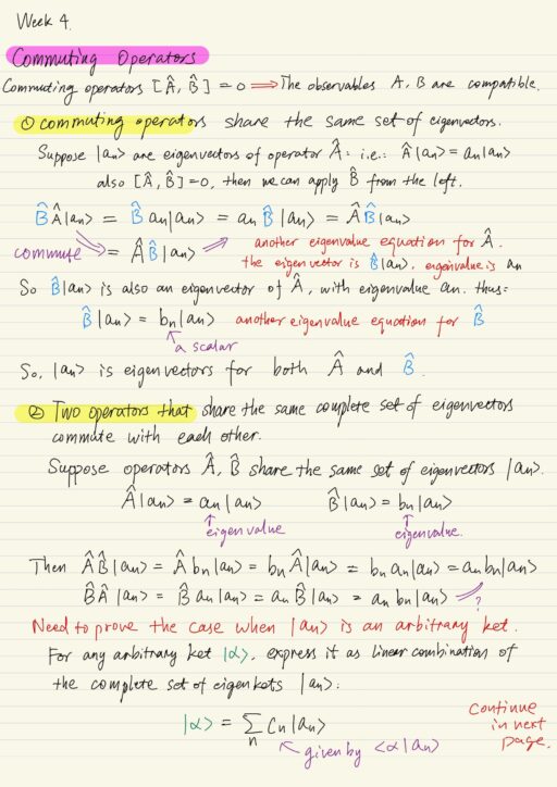
Commuting Operators

Two observables A and B are considered ‘compatible’ if the corresponding operators commute with each other, i.e.: [A^, B^] = 0, where [ ] is commutator bracket, and A^{^}, B^{^} are operators representing the physical observables A and B.

Commuting operators have two very important properties:

1. Commuting operators share the same set of eigenvectors.
2. The converse is also true: two operators that that the same complete set of eigenvectors commute with each other.

A^ B^|α⟩ = B^ A^|α⟩ ⟺ [ A^, B^ ] = 0 ⟺ A^ |an⟩ = an |an⟩, B^ |an⟩ = bn |an⟩

---

---

Recall a measurement does not alter the quantum state If the system was initially in one of the eigenstates of the operator representing the measured variable, or observable. Making two successive measurements of quantities whose operators commute or not, will exhibit different behavior.

If operators commute:

The first measurement collapses the system into one of its eigenstate, which is also an eigenstate of the second operator. Therefore the second measurement will not change the eigenstate. We know exactly what value we will measure with the second measurement.

If operators do not commute:

The first measurement collapses the system into one of its eigenstate, but that is NOT an eigenstate of the second operator. Therefore the second measurement will collapse the quantum system into its own eigenstate, which is distinct from the eigenstates of the first operator. We have inherent uncertainty we do not know exactly what value we will measure, we can only speak of probabilities of measuring certain values.

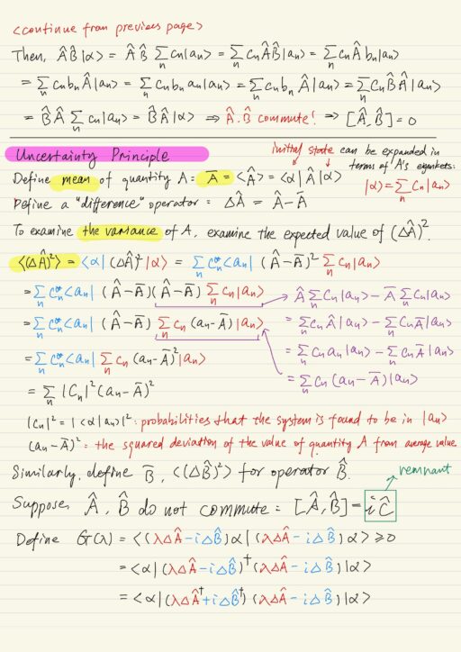
Uncertainty Principle

Let us use A^– to denote the mean value (expectation value) of quantity A, which is represented by Hermitian operator A^{^} and α is the initial state of the quantum system.

A- = ⟨A^⟩ = ⟨α| A^ |α⟩

Let us further define a new operator ∆A^{^} associated with the difference between the measured value of A and its average value. A- is only a real number, so ∆A^{^} is also Hermitian.

∆A^ = A^ - A-

Recall that the definition of variance of a random variable X is the expected value of the squared deviation from the mean of X: Var(X) = E[ ( X - E[X] )2 ]. To examine the variance of the quantity A, we examine the expectation value of the operator (∆A^)2.

⟨(∆A^)2⟩ = ⟨(A^ - A-)2⟩
= ⟨α| (A^ - A-)2 |α⟩
= ∑n |cn|2 (an - A-)2

⟨(∆A^)2⟩ is the mean squared deviation we will find for the quantity A upon repeatedly measuring the system whose initial state is |α⟩. We can similarly define the mean B- and variance ⟨(∆B^)2⟩ for another operator B^. Suppose A^ and B^ do not commute, i.e.: [ A^, B^ ] = i C^. The general form of the uncertainty principle is here, it tells us the minimum size of uncertainties in the measurement of two quantities. Perfectly certain measurements can be achieved only if the operators associated with the two quantities commute.

⟨(∆A^)2 (∆B^)2⟩ ≥ - (1/4) (⟨C^⟩)2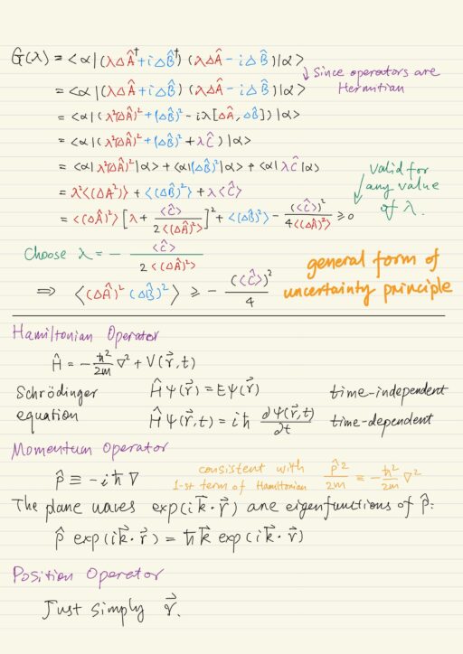

Hamiltonian Operator

Hamiltonian operator is defined as:

H^ = -(h2/2m) ∇2 + V(r→, t)

Adopting this definition, the time-independent Schrödinger equation can be written in a compact form as an eigenvalue equation

H^ ψ(r→) = E ψ(r→)

In non-relativistic quantum mechanics, the Hamiltonian operator is the operator related to the total energy of the system. Hamiltonian operator is also related to the time evolution of quantum states, as shown in the time-dependent Schrödinger equation:

H^ Ψ(r→, t) = i h ∂Ψ(r→, t)/∂t

Momentum Operator

The momentum operator postulated to be:

p^ ≡ -i h ∇ 

With this definition, the first term of Hamiltonian is consistent with the classical definition of kinetic energy p^2/2m ≡ -(h2/2m)∇2.

The plane waves exp(i k→ ∙ r→) are the eigenfunctions of the operator p^ with eigenvalue h k→.

p^ exp(i k→ ∙ r→) = h k→ exp(i k→ ∙ r→)

This is consistent with the De Broglie’s matter wave hypothesis p→ = h k→.

Position Operator

The postulated position operator is almost trivial in the framework of using wave functions of positions to describe quantum states. it is simply the position vector r→ itself. It is thus commonly written as just r without the hat symbol. The operator for the z-component of position would also simply be z itself.

---

---

Momentum-position uncertainty

Consider the commutator of the x-component of momentum p^x and position operator x, and apply that to an arbitrary |α⟩, we get:

[p^x, x] |α⟩ = -i h |α⟩

Compare [p^x, x] = -i h with the general form [A^, B^] = i C^, we get C^ = -h. According to the general uncertainty, we could get:

(∆px)2 (∆x)2 ≥ h2/4
⟹ ∆px ∆x ≥ h/2 ⟹ ∆kx ∆x ≥ 1/2

Diffraction

The momentum-position uncertainty is well-known in wave theory. Diffraction by a slit produces a divergent beam. The smaller the slit width is, the more divergent the beam is emerging from it.

The slit width defines the uncertainty of position, narrow slit means small uncertainty in position, that leads to a very large uncertainty in momentum along that direction, and that leads to a diverging beam.

Energy-time uncertainty

Consider t as time operator, use time-dependent Schrödinger equation then the commutator of H^{^} and t is:

[ H^, t ] = i h

Then we obtain:

(∆E)2 (∆t)2 ≥ h2/4
⟹ ∆E ∆t ≥ h/2

Frequency-time uncertainty

Since E = h ω, and ∆E ∆t ≥ h/2 leads to the famous frequency-time uncertainty in Fourier analysis.

∆ω ∆t ≥ 1/2

One can not simultaneously have both well-defined frequency and well-defined time for a signal. When a signal is a short pulse, it is necessarily contains a range of frequencies and vice versa. The minimum frequency bandwidth for a given time interval is determined by the same uncertainty relation.

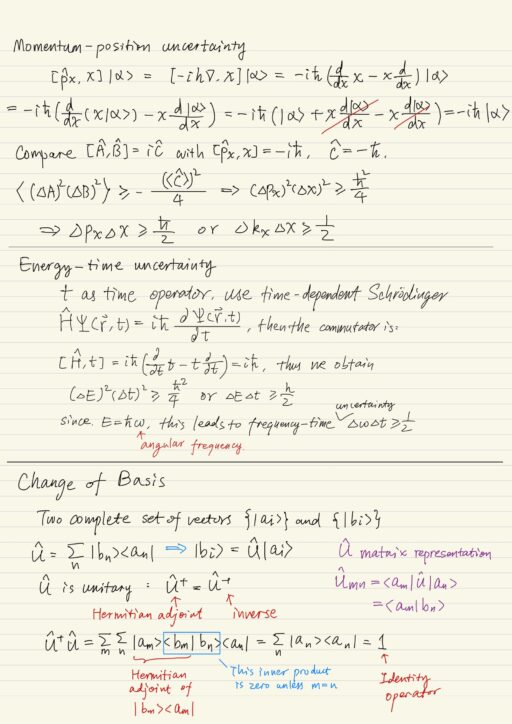
Change of Basis

We define a unitary transformation which allows us to transform one basis set to another. A convenient choice for basis set is the set of eigenvectors of a Hermitian operator, which are orthonomal and complete. But in general there are many choices for the basis set.

Two orthonormal complete sets of vectors { |a_i⟩ } and { |b_i⟩ } are related to each other by a unitary transformation, which results |bi⟩ = U^ |ai⟩:

U^ = ∑n |bn⟩⟨an|

Further more, U^ is unitary U^† = U^-1.

The matrix representation of U^ is Umn = ⟨am| U^ |an⟩ = ⟨am|bn⟩.

Transform vectors

Given column vector |α⟩, its representations in old basis ⟨an|α⟩ and new basis ⟨bm|α⟩ are related as below:

⟨bm|α⟩ = ∑n ⟨bm|an⟩ ⟨an|α⟩
= ∑n ⟨am|U^†|an⟩ ⟨an|α⟩ 

Transform operators

Similarly, transformation of matrix of an operator from old basis |ai⟩ to new basis |bi⟩ can be expressed as:

⟨bm|A^|bn⟩ = ∑k ∑l ⟨bm|ak⟩ ⟨ak|A^|al⟩ ⟨al|bn⟩
= ∑k ∑l ⟨am|U^†|ak⟩ ⟨ak|A^|al⟩ ⟨al|U^|an⟩

One important quantity that is preserved through the similarity transformation is the trace:

Tr(A^) = ∑n ⟨an|A^|an⟩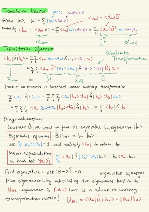

---

---

Diagonalization

Unitary transformation is fundamental related to the problem of finding eigenvalues of an operator or equivalently diagonalizing a matrix. Consider an operator B^, for which we want to find the eigenvalue bn and eigenkes |bn⟩, that satisfy the eigenvalue equation B^ |bn⟩ = bn |bn⟩. The matrix representation using the basis set {|ai⟩} of this eigenvalue equation is:

∑k ⟨am|B^|ak⟩ ⟨ak|bn⟩ = bn ⟨am|bn⟩

The eigenvalues can be found from the secular equation det(B^ - λ I^) = 0. Then you find the corresponding eigenvectors by substituting the eigenvalues λ back into the eigenvalue equation. Note that the eigenvectors in {|ai⟩} basis are simply columns in the unitary transformation matrix.

Umn = ⟨am|U^|an⟩ = ⟨am|bn⟩

If you express the operator B^ in its eigenvectors {|bi⟩} as the new basis set, the resulting matrix will simply be a diagonal matrix with the diagonal elements being the eigenvalues.

⟨bm|B^|bn⟩ = bnδmn

Wavefunctions in Position and Momentum Basis

More than being discrete, eigenvalues could be continously varying, for example: the energy in the potential barrier problem, or the momentum of a particle in free space. In these cases, most of the results from the discrete cases are readily extended by changing the sum ∑ to integral ∫. Consider an eigenvalue equation with continuous spectrum of eigenvalue:

ξ^ |ξ⟩ = ξ |ξ⟩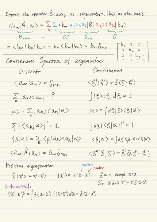

Position eigenfunction

Position eigenfunction should satisfy the eigenvalue equation, where x^ is the position operator, which equals to x in the position basis. x' is the eigenvalue. |x'⟩ is the eigenket, which is actually a delta function δ(x - x').

x^ |x'⟩ = x' |x'⟩

The delta function (eigenfunctions) are also orthonormal ⟨x' | x''⟩ = δ(x' - x'').

Momentum eigenfunction

Recall momentum operator is p^x = - i h ∂/∂x. To satisfy the eigenvalue equation, the fully normalized eigenfunction is ψk(x) = 1/√(2π) exp(ikx) in the position basis set, with eigenvalue hk.

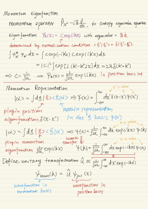
Momentum representation

The wavefunction ψ(x) is really the representation of |α⟩ in the position basis set.

Position eigenfunction:

In position basis	In momentum basis
ψpos(x) = δ(x – x0)	ψmom(k) = 1/√(2π) exp(- i k x0)

Momentum eigenfunction:

In position basis	In momentum basis
ψpos(x) = 1/√(2π) exp(i k0 x)	ψmom(k) = δ(k – k0)

We can also present position operator in momentum basis:

x^mom = i h ∂/∂p

and similarly present momentum operator in position basis:

p^pos = - i h ∂/∂x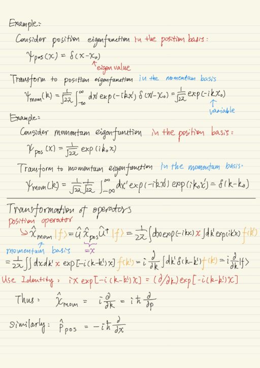

---

---

My Certificate

For more on Quantum Mechanics: Uncertainty Principle and Change of Basis, please refer to the wonderful course here https://www.coursera.org/learn/foundations-quantum-mechanics

My #83 course certificate from Coursera

---

Related Quick Recap

Stern-Gerlach Experiments & Dirac Bra-ket Notation

---

I am Kesler Zhu, thank you for visiting my website. Check out more course reviews at https://KZHU.ai

Don't forget to sign up newsletter, don't miss any chance to learn.

Or share what you've learned with friends!

Tweet