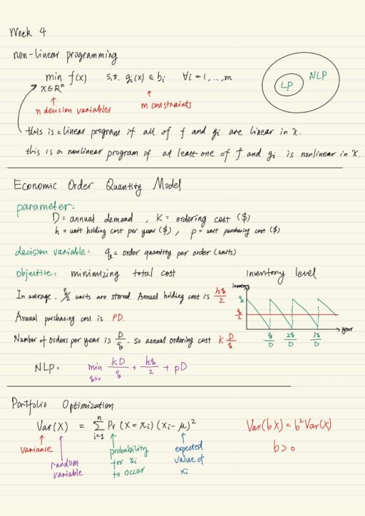
In many cases, we need to deal with nonlinear situations, e.g.: product pricing decision, inventory, portfolio optimization. Above all, the purpose is to find a balance between tradeoffs. Usually non-linear programs are more general than the linear programs. Formulating non-linear program is usually easy because you rarely use weird constraints; but its optimization would be hard.
Economic Order Quantity (EOQ) Model
The EOQ model helps us make the order quantity decision, which is the most economic. It is actually looking for a balance between the ordering cost and holding cost. Typically we formulate an non-linear program whose solution is the optimal order quantity. There are a few assumptions of EOQ model:
- The demand is deterministic and consumption rate is constant.
- The ordering cost is fixed, regardless of the quantity ordered.
- No shortage is allowed.
- The ordering lead time is zero.
- The inventory holding cost is constant.
The key to formulate the problem is to understand how inventory level is affected by our decision.
Portfolio Optimization
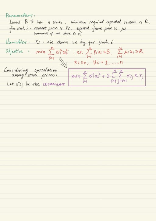
There are plenty of ways to measure risk. Markowitz and Sharpe suggest the total revenue is random, the larger the variance of the total revenue, the higher the risk. So we want minimize the total variance while ensuring a certain expected revenue. We want to use the method with lowest risk to guarantee some expected revenue. Given different value of expected revenue, we get different optimal portfolios.

Linearization
| Linear program | easy |
| Linear integer program | doable |
| Non-linear program | hard |
| Non-linear integer program | very hard |
Many nonlinear functions can be linearized through the help of binary variables.
Linearization of Max and Min
Absolute value functions
Absolute value functions are nonlinear. It can be linearized as follows:
- First use a variable to present the absolute value, say
w = | x |. - Then we could move the absolute value function from objective function to constraints.
- Next changing equality to inequality, say changing
w = | x |tow ≥ | x |. This will change the feasible region, but won’t change the optimal solution. Because if there are values satisfy the strict inequality ( the > part of ≥ ), there are always room to get a smaller possible number, so the original solution can not be optimal. If there is an optimal solution, the optimal solution will make the inequality binding ( the = part of ≥ ). - Essentially, absolute value function can be expressed as the maximum of two terms:
| x | = max { x, -x }, which makesw ≥ | x |equivalent tow ≥ max { x, -x }, which is further equivalent tow ≥ xandw ≥ -x. It means w would be lower bounded by the greater of x or -x .
| original | linearization |
| min | x | | min w s.t. w ≥ x and w ≥ -x |
Min and max functions in constraints
The technique we applied previously can be generalized, because the linearization is based on logic AND:
| Condition | Original | Linearization |
| When max function is at the smaller side of inequality | y ≥ max { xi } i = 1,…,n | y ≥ xi for any i = 1,…,n |
| When min function is at the larger side of inequality | y ≤ min { xi } i = 1,…,n | y ≤ xi for any i = 1,…,n |
The linearization above can not apply to these situations:
- When max function is at the larger side of inequality
- When min function is at the smaller side of inequality
- When max or min function in an equality
In the situation 1 and 2 above, the logic is OR (instead of AND). The linearization of this can be accomplished using binary variable, but this will introduce integer programming which is complicated and inefficient.
Min and max functions in objective functions
| Original | Linearization |
| min max { xi } + yi s.t. other constraints | min w + yi s.t. w ≥ xi and other constraints |
| max min { xi } + yi s.t. other constraints | max w + yi s.t. w ≤ xi and other constraints |
This technique can not be used with min min or max max.
Absolute value function revisited
Based on discussions above, absolute value function is just a max function | x | = max {x, -x}, so it can be linearized when:
- minimizing an absolute value function.
- absolute value function is at the smaller side of an inequality.
Linearization of Products
The product of 2 decision variables can be linearized if any of them is binary. The product can not be linearized if both of decision variables are continuous.
Both decision variables are binary
If the products appear in objective function:
| Original | Linearization | Boundary for w |
| max x * y s.t. x, y ∊ {0, 1} | max w s.t. x, y ∊ {0, 1} w ≤ x w ≤ y w ∊ {0, 1} | upper |
| min x * y s.t. x, y ∊ {0, 1} | min w s.t. x, y ∊ {0, 1} w ≥ x + y – 1 w ∊ {0, 1} | lower |
If the products appear in constraints:
| Original | Linearization | Boundary for w |
| if x * y is at the larger side, treat x * y itself is a min function. max … s.t. z ≤ x * y x, y ∊ {0, 1} | linearize it as if it appears in a max objective function. max … s.t. z ≤ w x, y ∊ {0, 1} w ≤ x w ≤ y w ∊ {0, 1} | upper |
| if x * y is at the smaller side, treat x * y itself is a max function. max … s.t. z ≥ x * y x, y ∊ {0, 1} | linearize it as if it appears in a min objective function. max … s.t. z ≥ w x, y ∊ {0, 1} w ≥ x + y – 1 w ∊ {0, 1} | lower |
Only 1 of 2 decision variables is binary
If the products appear in objective function:
| Original | Linearization | Boundary for w |
| max x * z s.t. 0 ≤ x ≤ n z ∊ {0, 1} | when z = 1, let the upper bound is exactly x when z = 0, let the upper bound is 0 max w s.t. 0 ≤ x ≤ n z ∊ {0, 1} w ≤ x w ≤ n * z | upper |
| min x * z s.t. 0 ≤ x ≤ n z ∊ {0, 1} | when z = 1, the lower bound is x when z = 0, the lower bound is 0 min w s.t. 0 ≤ x ≤ n z ∊ {0, 1} w ≥ x – n * ( 1 – z ) w ≥ 0 | lower |
If the products appear in constraints:
| Original | Linearization | Boundary for w |
| if x * z is at the larger side, treat x * z itself is a min function. max … s.t. y ≤ x * z 0 ≤ x ≤ n z ∊ {0, 1} | linearize it as if it appears in a max objective function. max … s.t. y ≤ w 0 ≤ x ≤ n z ∊ {0, 1} w ≤ x w ≤ n * z | upper |
| if x * z is at the smaller side, treat x * z itself is a max function. max … s.t. y ≥ x * z 0 ≤ x ≤ n z ∊ {0, 1} | linearize it as if it appears in a min objective function. max … s.t. y ≥ w 0 ≤ x ≤ n z ∊ {0, 1} w ≥ x – n * ( 1 – z ) w ≥ 0 | lower |
My Certificate
For more on Operations Research: Nonlinear Programming and Linearization, please refer to the wonderful course here https://www.coursera.org/learn/operations-research-modeling
Related Quick Recap
I am Kesler Zhu, thank you for visiting my website. Check out more course reviews at https://KZHU.ai
