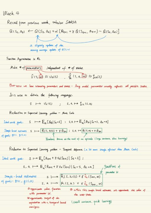
Deduction to supervised learning problem
In tabular method, each Q(s, a) could be seen as a parameter. There are more parameters than states, because there are as many parameters for each state as the possible number of actions for each state. There are also situations where states include continuous components. It means we need a table of infinite size.
In these situations we need to approximate and generalize the unseen and closed states. Ideally we would want to make number of parameters independent of the number of states. We want to approximate (state-)value function and action-value function using some parametric model V^ and Q^. Monte Carlo usually has large various due to lots of random variables, and learn slowly. On the other side, the Temporal Difference with small variance learns faster.
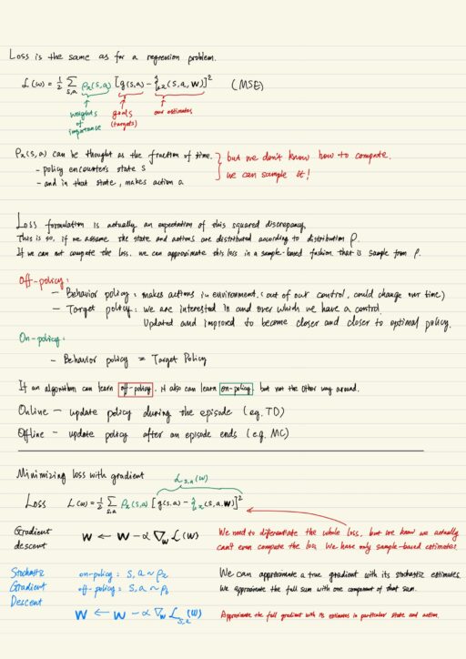
For loss function, it is natural to impose a regression loss for q-learning. There are plenty losses for regression task, either MSE or MAE works. We are interested in accurate estimation of Q-function in some states, and are almost indifferent in the Q-function for some other states. Because the estimate of each state and action could only be improved only after experiencing that state and taking that action, but no body want agent to experience bad states and make bad actions, over and over again just to improve the precision of bad action estimates. So we multiply the discrepancy with “weights of importance”
Loss formulation is actually an expectation of this squared discrepancy. This is so if we assume the state and action are distributed according to “weights of importance”. If we can not compute the loss, we can approximate the loss in a sample-based fashion, that is sample from “weights of importance”.
Loss function
Once we have the loss function, we might want to minimize it. The most simple and widespread method is gradient descent. It is differentiating the loss with respect to the parameter w, and change parameter w in the direction of minus gradient multiplied with some step size (alpha). We need to differentiate the whole loss, but we know we actually can’t even compute the loss, we have only sample-based estimates. In SGD, approximate a true gradient with its stochastic estimates. We approximate the full gradient with its estimates in particular state and action.
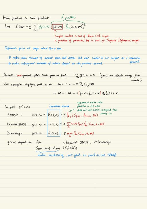
Taking derivative of goal function will cause many problems, so we employ stochastic semi-gradient descent. The properties of semi-gradient include:
- Treats goal function g(s, a) as fixed numbers.
- Like gradient update, it updates parameters in a way that moves estimates to targets.
- Unlike gradient update, it ignores effect of updates on targets.
- Semi-gradient is not a proper gradient
- it does not possess convergent properties of stochastic gradient descent
- it converges reliably in most cases
- more computationally efficient than stochastic gradient descent
- A meaningful type of parameter update correspond to symmetric structure of tasks that time goes only forward.
Difficulties with approximate methods
The most obvious one is “curse of dimensionality”. That is the number of state-action pairs grow exponentially with the number of variable which is used to describe them. We should use methods which are sufficiently sample-efficient. We also need these methods to be flexible to make accurate estimates and meaningful decisions. Any model has finite number of parameters, which limits the model even though it is a universal approximator. Finally there are the common issue like over-fitting and under-fitting.
Problems with Supervised Learning in RL
FIrst, in Reinforcement Learning, data is usually highly correlated and non-IID (independent and identical distributed). The change in environment will not only make agent forget facts and features, but also force it to learn from scratch. Very many methods in supervised learning rely heavily on the data being IID. When this is not the case, learning can be either inefficient or break down completely. At last Stochastic gradient descents can lose convergence properties in the case of non-IID.
Second, data usually depends on current policy. Besides actions chosen by policy, states and rewards are also influenced by policy. When we update the parameter of policy, we change actions, states and rewards. Unseen data comes as agents learn new things. Agent can learn fatal behavior and new data is insufficient to unlearn it.
Third, Q(s, a) often change abruptly in change of s, a. Close states could be arbitrarily far in value. Successive states could be arbitrarily far in value. All this leads to unstable gradient and data inefficiency. Besides that, if you use Temporal Difference, error in estimates propagates.
Non-stationarity in Generalized Policy Iteration
All algorithms in RL are actually “Generalized Policy Iteration”. We constantly update estimates, that are defined with policy. When we change policy, we actually invalidate estimates of Q-values. This inherent non-stationarity can in turn cause problems like oscillating behavior.
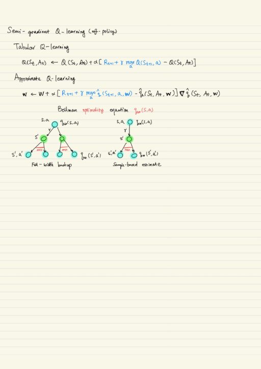
Deadly triad – model divergence
If we add these ingredient together, we may get an algorithm which may diverge.
- Off-policy learning. Learning target pi while following behavior b.
- Bootstrapping. Updating a guess towards another guess. (TD, DP)
- Function approximation (using model with number of parameters smaller than number of states)
How ever if we remove any of the 3 ingredients, no divergence is possible.
My Certificate
For more on supervised learning in reinforcement learning, please refer to the wonderful course here https://www.coursera.org/learn/practical-rl
Related Quick Recap
I am Kesler Zhu, thank you for visiting. Check out all of my course reviews at https://KZHU.ai
