Risk Management: Equity Derivatives in Practice

Table of Contents

Review of Self-Financing Trading Strategy

A self-financing trading strategy is a trading strategy θ_t = (x_t, y_t) where changes in V_t are due entirely to trading gains or losses, rather than the addition or withdrawal of cash funds. Why do we care?

Dynamic Replication: in the multi-period binomial model, we can actually construct a self-financing trading strategy that replicates the payoff of any derivative securities. The cost of this replicating strategy must equal to the value of the security, otherwise there is an arbitrage opportunity. The dynamic replication price is of course equal to the price obtained from using the risk-neutral probabilities and working backwards in the lattice.

Review of Black-Scholes Model

Black and Scholes assumed:

a continuously compounded interest rate of r.
Geometric Brownian motion dynamics for the stock price S_t.
The stock price is assumed to pay a dividend yield of c.
Continuous trading without transactions costs and short-selling is allowed.

Binomial model can be viewed as an approximation of Geometric Brownian motion. If number of periods n -> infinite then binomial paths will looks like Brownian paths.

Note the drift μ does not appear in the Black-Scholes formula, just as p (true probability) is not used in the option pricing calculations for the binomial model. The call option price in the Black-Scholes model actually depends on S₀, K, T, r, σ, c. But μ does enter implicitly into the value of the call option.

Black-Scholes Geometric Brownians Motion model is not a good approximation to security prices.

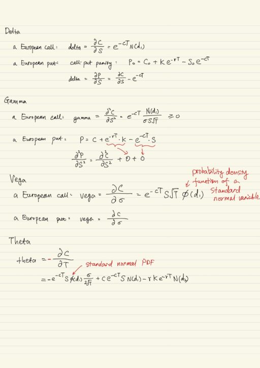
Delta, Gamma, Vega and Theta

“Greeks” refer to the partial mathematical derivatives of a financial derivative security price with respect to the model parameters.

Delta	The partial derivative of the option *price* with respect to the price of the underlying security.
Gamma	The partial derivative of the option’s *delta* with respect to the price of the underlying security.
Vega	The partial derivative of the option price with respect to the *volatility parameter σ.*
Theta	The *negative* of the partial derivative of the option with respect to *time-to-maturity T.*

Approximation to Option Prices

Taylor’s Theorem enables us to see what happens to the call option price for small changes in price S and small changes in volatility σ. The profit and loss (P&L) on the option price, when the stock price changes by an amount of ΔS and the volatility changes by an amount of Δσ, will be equal to a delta component plus a gamma component plus a vega component, and optionally plus a theta component. This is often used in historical Value-at-Risk VaR calculations.

Investors often know what equivalent stock position (ESP) is, what $Gamma is, and vega of their option. Knowing these quantities will help them understand how their portfolio behaves as the underlying stock moves and as the volatility parameter σ changes.

The P&L also applies to portfolios of derivatives. The Greeks are very useful. People understand their risk sensitivities in terms of these Greeks. But for very large move in S or σ, P&L can break down, it can no longer work. In that case, you should use scenario analysis.

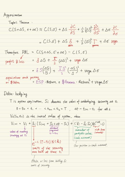
Delta-Hedging

Delta-hedging allows to exactly replicate the payoff of an option. We are following self-finance trading strategy whose value at maturity is exactly equal to the value of derivative that we are trying to replicate. Delta-hedging is possible in the context of the Black-Scholes model. However in practice we can not delta-hedge exactly because we can not trade at every instance in time, we don’t know the true model and the true parameters of the model. So it can only be done approximately.

In the Black-Scholes model and option can be replicated exactly by following a self-financing trading strategy. Recall that binomial model can be approximation of geometric Brownian motion. As periods of n goes to infinity, the binomial model converges in an appropriate sense to geometirc Brownian motion. Therefore it should not be surprising that it is also the case in the Black-Scholes model that every security can be replicated exactly by following a self-financing trading strategy. When we execute the strategy, we say we are delta-hedging the option.

In practice you can not trade continuously, and you have to pay transaction costs. We can no longer exactly replicate the option payoff, we have to approximately replicate the option payoff. The volatility σ parameter must be correct, but in practice we can not expect to know it. If we assume the wrong σ, then V₀ and all δ_i will be wrong.

We don’t know σ, and the true dynamics of the security prices don’t follow geometric Brownian motion, so the concept of dynamic replication is really only a theoretical concept. If we guess σ correctly, we can hope to replicate the option approximately and sufficiently accurate for risk management purposes.

Volatility Surface

If the Black-Scholes model was correct, the volatility surface would be flat. In practice, it is anything but flat and move about randomly.

The Black-Scholes model is elegant but does not perform well in practice, the reasons include:

the security prices often jump, but this is not true with geometric Brownian model
the security prices tend to have fatter tails than those implied by log-normal distribution (the extreme returns are more likely)
returns are clearly not IID in practice

Market participants are well aware that Black-Scholes model is a pool approximation to reality. But it is still very necessary to understand the Black-Scholes model if you want to understand derivative’s pricing and how derivatives are used in practice.

The incorrectness of Black-Scholes model is most obviously manifested through the Volatility Surface, which is defined as a function of strike K and expiration T.

For a given expiration T, options with lower strikes tend to have higher implied volatilities, this feature is typically referred to as volatility skew or smile.
For a given strike K, the implied volatility can be either increasing or decreasing with time to maturity T. In general for a fixed K, σ(K, T) converges to a constant as T goes to infinity. Meanwhile when T is small, you often observe an inverted volatility surface, with short term options have much larger volatilities than long term options. Option prices increase with volatility, so when there is a market stress, we tend to see short-term options have much larger volatilities than longer maturity options.

Single stock options are generally American, in this case, call and put options generally give rise to different surfaces.

Arbitrage Constraints

The shape of volatility surface is constrained by the absence of arbitrage. In particular:

σ(K, T) >= 0 for all K, and T.
for any T, the skew can not be too steep, otherwise arbitrage opportunities (such as a put spread arbitrage) would exist.
the term structure of implied volatility can not be too inverted, otherwise arbitrage opportunities (such as calendar spread arbitrage) would exist.

In practice, implied volatilities will not violate any of these restrictions, but these restrictions can be difficult to enforce when we are stressing the surface, which is used often in risk management applications.

Volatility Skew

There are at least 2 principle excuses for the skew:

Risk aversion, this can appear in many guises
- Security prices jump to downside more frequently than upside.
- As market goes down, fear and panic sets in and volatility goes up
- supply and demand
Leverage effect, the total value of company assets (debt + equity) is a more natural candidate to follow geometric Brownian motion, or at least to have IID returns.

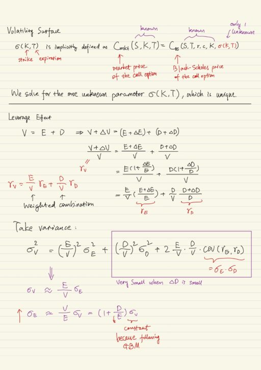
Leverage Effect

The fundamental accounting equation states V = D + E. V is total value of a company, D is company’s debt, E is company’s equity. Merton recognized that equity E could be viewed as a call option on V with strike equal to D, because debt holders get paid before equity holders.

E = max(0, V - D)

Equity is the riskiest part of the capital structure of a company. Equity holders actually incur losses before debt holders. We could first let V (instead E) follow geometric Brownian motion, then use risk-neutral pricing to actually get the value of the equity E, and then get the value of debt D as well. This give rise to the “structural models” for pricing the components of the capital structure in a company.

Suppose that the equity E is substantial, so that it absorbs almost all the losses or gains, and debt D is not risky, so ΔD will be small, and therefore debt volatility σ_D can be ignored. We can derive and get the following equation.

σ_E ≈ ( 1 + D / E ) * σ_V
σ_E is equity volatility
σ_V is asset value volatility

We suppose asset value follows geometric Brownian motion, so σ_V is a constant; as E or V goes up or goes down, σ_E will change accordingly. So σ_V is constant, but σ_E is stochastic.

Pricing Derivatives

Volatility surface tells us the marginal risk neutral distribution of the stock price at a given fixed time, it gives us nothing about the joint risk neutral distribution of the stock price at various times. Volatility surface is certainly used for risk management purposes.

Given the implied volatility surface σ(K, T) we can compute the price P₀ of any derivative security whose payoff f only depends on the underlying stock price S_T at a single and fixed time capital T.

P₀ = E₀^Q [e^-rT f(S_T)]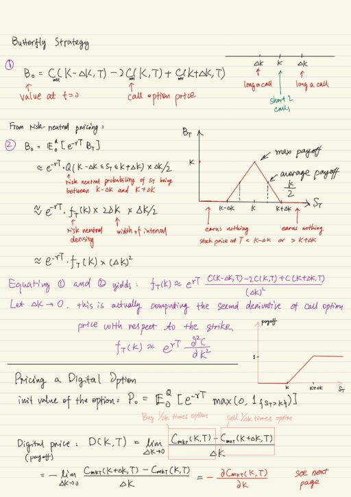

Pricing a Digital Option

Digital option pays $1 if the time T stock price S_T is greater than K and pays $0 otherwise. We can actually price the security given the implied volatility surface, because as long as you know implied volatility surface, you know the marginal risk-neutral distribution of the security price at a fixed time T. So the payoff of this option is:

max(0, 1_{{ST > K}})

The risk neutral distribution of this option only depends on the marginal risk neutral distribution of S_T. So we can evaluate the initial value of this digital option by:

E₀^Q [e^-rT max(0, 1_{{ST > K}})]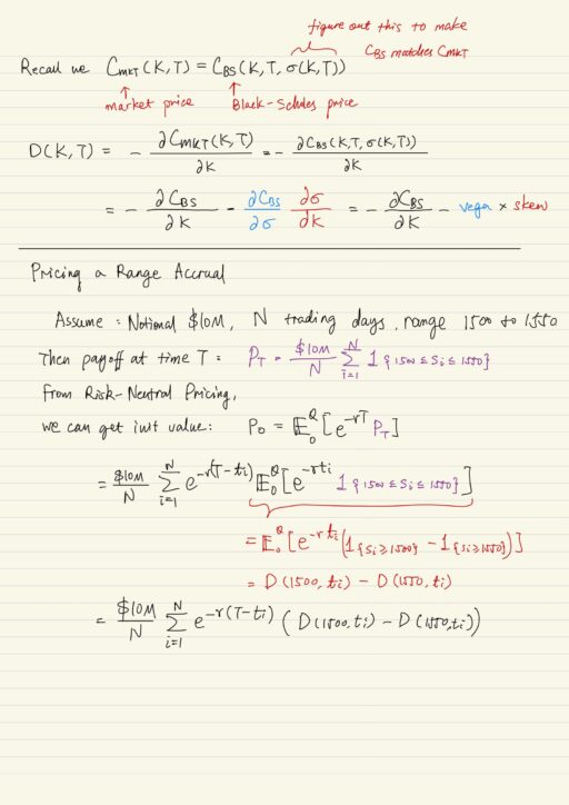

Pricing Range Accrual

An M-month range accrual product pays X% of notional where X equals to the percentage of days over M-month that price/index is inside a range. For example, if notional is $10M, and the index is inside the range 70% of the time, then the payoff is $7M.

Volatility surface can help calculate the price of this range accrual, considering a portfolio consisting of a pair of digital’s for each date between now and the expiration.

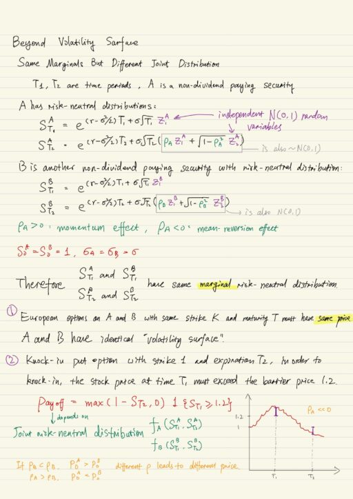
Beyond Volatility Surface

There are many derivative securities that can not be priced using volatility surface, because the price of these derivative securities depend on the joint risk-neutral distribution of the stock price at multiple times, for example: the barrier options.

The dynamic replication theory of Black-Scholes is very elegant but it is not possible to dynamically replicate (and therefore price) derivative securities in practice, because:

Securities prices don’t follow geometric Brownian motions.
You can not trade continuously
Avoiding transactional costs is impossible

So dynamic replication is something we can only approximate. Instead supply and demand is what sets derivative security prices. Indeed volatility itself is an asset class, because people want to trade volatility. It is possible to buy volatility by buying a European call or put option, whose value will increase when its volatility increases.

That having been said, derivative pricing models are still needed to:

price exotic and other less liquid derivative securities.
risk-manage derivatives portfolios via the Greeks or scenario analysis

My Certificate

For more on Risk Management: Equity Derivatives in Practice, please refer to the wonderful course here https://www.coursera.org/learn/financial-engineering-2

My #69 course certificate from Coursera

Financial Engineering: Implementing Mean-Variance

I am Kesler Zhu, thank you for visiting my website. Checkout more course reviews at https://KZHU.ai

Don't forget to sign up newsletter, don't miss any chance to learn.

Or share what you've learned with friends!