Non-Linear Programming: Gradient Descent and Newton’s Method

Tweet

Non-Linear Programs

When visualizing a linear program, its feasible region looks like a polygon. Because the objective function is also linear, the optimal solution is on the boundary or corner of the region.

But a non-linear program is quite different, its feasible region may be in any shape, moreover the optimal solution may not exist on the boundary of the feasible region. Searching the whole feasible region does not work particularly when there are hundreds or thousands of variables.

---

---

A better idea is to use derivative at a point to tell us what is gonna happen if we move in certain direction. Suppose a non-linear objective function y = y(x) with only one variable x. At point x₀, if the derivative is positive, we will know y will decease if x decreases, and y will increase if x increases. Then ask the question: around all my feasible directions, where should I go to reach my target as soon as possible? The answer really depends on the derivative.

The program we want to solve usually contains multiple variable, so a single derivative is not enough, we need derivatives along all the directions, which is the concept of gradient from vector calculus. Gradient descent is a very popular algorithm of solving non-linear problems. Gradient descent is actually first-order approximation, Another more powerful method is Newton’s method, which is essentially second-order approximation.

We rely on numerical algorithms for obtaining a numerical solution. Solving a nonlinear program usually in the following ways:

Iterative	In many cases we have no way to get to an optimal solution directly, we need to move to a point in one direction and then starts the next iteration search starting from that point.
Repetitive	In each iteration, we repeat the same steps.
Greedy	In each iteration, we seek for some best thing achievable in that iteration.
Approximation	Rely on the first-order or second-order approximation of the original program.

Nonlinear programs are harder than linear programs, so finding solutions for them may fail due to many reasons:

1. Fail to converge to a single point, you won’t get a feasible solution at all.
2. Trapped in local optimum, which means starting point matters.

It is usually required that the objective function’s domain is continuous and connected. If that is not true, we are probably dealing with nonlinear integer program, which is too hard to solve – gradient descent and Newton’s method will fail, more advanced topics like Convex Analysis may be required.

Unconstrained non-linear programs are in some sense easier to solve than constrained ones:

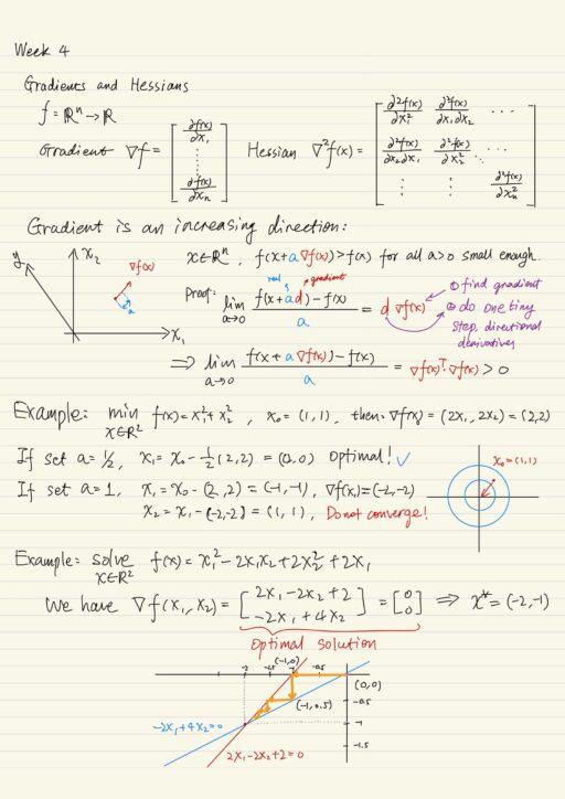
minx ∈ Rn f(x), where f is a twice-differentiable function

Gradients and Hessians

For a function f: Rn → R, collecting its first- and second-order partial derivatives generates its gradient ∇f(x) and Hessian ∇2f(x).

Gradient Descent

At any point of the domain of the function x ∈ Rn, we consider its gradient ∇f(x), which is an n-dimensional vector. Gradient is closely related to slope ∆f(x)/∆x only in 1-dimensional problem, but this is not true in general. In n-dimensional space, the gradient actually is the fastest increasing direction where if you move along that direction.

f(x + a ∇f(x)) > f(x), for all a > 0 that is small enough

We may try to “improve” our current solution x by leveraging gradient. Since we are minimizing the function f(x), here “improve” mean we want to get to a lower value of f(x), we first find the gradient, then we move along the opposite direction.

Suppose current solution is x, in each iteration we update x using gradient ∇f(x) and step size a, until gradient becomes or very close to 0.

x = x - a ∇f(x), a > 0 

Selecting appropriate value of step size a is critical, a few strategies include:

1. Predefine step size and decreasing it gradually.
2. Look for the largest improvement and then select appropriate value of step size.

Now the pseudo code of the gradient descent algorithm using adapted step size:

1. Set k = 0, choose starting point xk and precision parameter ε > 0.
2. Find gradient ∇f(xk)
3. Solve ak = argmina ≥ 0 f(xk - ak ∇f(xk))
4. Update current solution xk+1 = xk - ak ∇f(xk)
5. If the norm of the gradient || ∇f(xk+1) || < ε, exit
6. Increase k = k + 1, and go to step 2

When we want to apply gradient descent in this particular manner, always, we need to formulate a sub-problem of step size a, which is also a minimization problem, finding the first-order condition such that the step size a can minimize the objective value. We know that what our algorithm is doing is to search only one direction (one variable) at a time, until finally we are getting close to the optimal solution. When you do gradient descent, you pretty much always go in zig zag with right angles.

---

---

Newton’s Method

Newton’s method is similar to gradient descent. In each iteration, it tries to move to a better point. But gradient descent is first-order method and too slow sometimes. Newton’s method is second-order method which relies on the Hessian to update a solution.

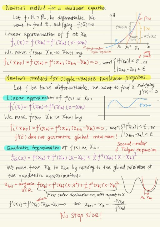
For non-linear equations

Suppose a non-linear differentiable function f, we want to find x* that satisfies f(x*) = 0. Starting from a initial point x0, consider the linear approximation of the function f(x) at that point. We are actually using Taylor expansion to create linear relaxation fL(xk+1) of f(x) at point xk (moving from x_k to x_k+1):

fL(xk+1) = f(xk) + f'(xk) (xk+1 - xk) = 0

We don’t really directly solve our non-linear problem for this nonlinear equation f(x), maybe we don’t know how to solve it, but for the linear relaxation fL(x), everything is so easy. Continue the iteration until either |f(xk)| < ε or |xk+1 - xk| < ε, where ε is a very small number.

For single variate non-linear programs

If we have a twice-differentiable function f(x) where there is a minimum point, at that point we must satisfy the fact that the gradient ∇f(x) must be 0. We use linear approximation of f'(x), i.e. the derivative of f(x), to move from x_k to x_k+1 to approach the root x*.

f'L(xk+1) = f'(xk) + f''(xk) (xk+1 - xk) = 0

Continue the iteration until either |f'(xk)| < ε or |xk+1 - xk| < ε, where ε is a very small number. Note f'(x*) does not guarantee a global minimum. It may be a local min, or even a local max.

Another interpretation is to use quadratic approximation of f(x) at x_k, and move from x_k to x_k+1 by moving to the global minimum of the quadratic approximation:

xk+1 = argminx∈R f(xk) + f'(xk) (x - xk) + (1/2) f''(xk)(x - xk)2

This is actually equivalent to solving ∇f(x) = 0. Note that if your function looks weird, then this approach may fail – what you want is to find a lower objective value, but actually after one iteration, you get a value higher. Newton’s method does not guarantee you improvement in each iteration.

For nice behavior functions, Newton’s method may be faster than gradient descent, but gradient descent is a much more robust algorithm. Gradient descent always do meaningful search unlike Newton’s method. 

For multi-variate non-linear programs

All we need to do is to generalize the idea of single dimensional derivatives to gradients and Hessians. The quadratic approximation of f(x) at x_k:

fQ(x) = f(xk) + ∇f(xk)T (x - xk) + (1/2) (x - xk)T ∇2f(xk) (x - xk)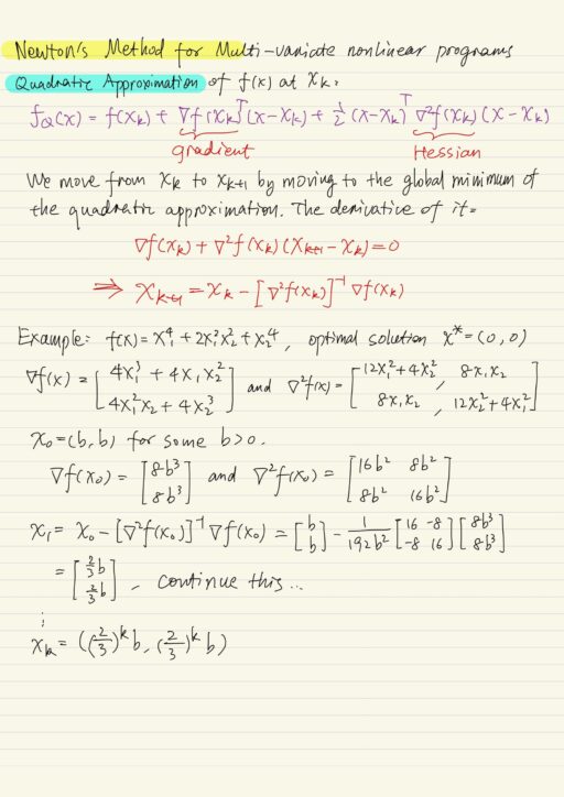

---

---

My Certificate

For more on Non-Linear Programming: Gradient Descent and Newton’s Method, please refer to the wonderful course here https://www.coursera.org/learn/operations-research-algorithms

My #82 course certificate from Coursera

---

Related Quick Recap

Branch-and-Bound & Heuristic Algorithms

---

I am Kesler Zhu, thank you for visiting my website. Check out more course reviews at https://KZHU.ai

Don't forget to sign up newsletter, don't miss any chance to learn.

Or share what you've learned with friends!

Tweet