There are many aspects of implementation details of mean-variance. 3 of them are the most important.
- Parameter estimation
- The true mean vector and the true covariance matrix of the assets is unknown. All we have is historical return data. As a consequence, we end up making statistical errors. But portfolio are very sensitive to these errors. Data is usually sufficient for estimating mean vector, but is never sufficient for estimating covariance matrix. It is because the covariance matrix has d2 independent parameters. In order to estimate them, you have to collect return data over a very long period, but during which the market parameters shift. So you will never be able to get enough data.
- Negative exposure
- Very often the optimal portfolio has short positions. Taking on short positions is very dangerous and often not allowed for wealth managers. One way to get negative exposure is to use a leveraged Exchange Traded Fund (ETF), but you also have to be very careful.
- Variance as Risk Measure
- It works for normal (or elliptic) random variables and needs higher moments to capture deviation from normality.
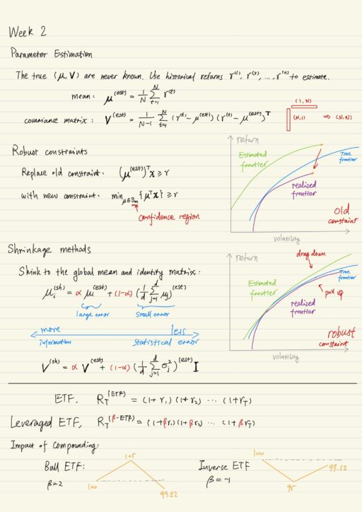
Parameter estimation
The estimated mean can be very far away from the true mean. True mean can lie in an ellipse with a certain probability. Parameter error is usually very serious for mean-variance portfolio selection. There is usually a big gap between the estimated return and the true return on the same portfolio. The estimated frontier is extremely unstable.
| Estimated frontier | frontier for estimated parameters |
| Realized frontier | frontier computed using true mean and volatility of the estimated frontier portfolio |
The problem of mean-variance portfolio selection is, after estimating these parameters, you will optimize portfolio using these parameters. Assets with larger estimated return will be over-weighted. If short position is allowed, then the assets with estimated smaller return will be sold, and then more is invested in the assets with the estimated larger return.
If this “optimized” portfolio is put into the market, you will get a return where over-weighted asset is going to perform worse than expected (the realized = μ, the expected = μ + ε), and under-weighted asset is going to perform better (the realized = μ, the expected = μ – ε).
Mean-variance results in error-maximizing investment-irrelevant portfolios.
Ron Michaud
Improvements with Optimization Strategies
No-short sales constraints
If short sales is not allowed, the realized frontier will be very unstable, there is a large part of the curve which is inefficient. The reason behind this, is the feasible region for the portfolio now has a corner. As you add more constraints (for example, how much money a sector can have), more corners and more instabilities are induced.
Leverage constraints
Leverage constrains is something like ∑di=1 |xi| ≤ 2. If we have leverage constraints, the gap between the realized frontier and the true frontier will be small, but the gap between the realized frontier and the expected frontier is still large. Leverage constraints do work well in practice, but still some more work needed.
Robust constraints
The robust portfolio selection removes the target return constraints (imposed with respect to the estimated value of mean), and replaces it by a target return constraint (with respect to the worse possible mean in the confidence region – an ellipse). It means you choose your portfolio x, the return that you are going to get is the worst possible return in the confidence region.
The worst possible return drags down the estimated frontier, getting close to the true frontier. The realized frontier is getting pulled up, so the gap between the expected frontier and the realized frontier is getting smaller. Sometimes you get portfolios which are not very interpretable, but overtime this technology is likely to be very practical.
Improvements with Estimation Strategies
Shrinkage methods
One shrinks to some global quantity. Let us take the case of the mean. In the past, I would estimated each of the asset’s mean separately μi(est), now I am also going to estimate a global average mean on the assets, assuming all the assets have the same estimated mean. As a result, I can expect the error in the global mean is smaller, and the error in larger in the individual mean.
Black-Litterman method
Use subjective views to improve estimates.
Non-parametric nearest neighbor-like methods
People started going away from parametric models like mean-variance and more going towards data-driven models.
Short positions
Short positions can result in very high returns, but it is also very risky.
- Long positions have limited downside, the largest amount one can lose is the amount invested.
- Short positions have unlimited downside, they are created by selling assets borrowed from a broker, and these have to be repurchased and returned to the broker at a later date. The potential loss can be arbitrary large.
So we need a product that has negative exposure, and limited downside, Exchange Traded Funds is one of them.
Exchanged Traded Funds (ETFs)
ETFs are exchange traded product that tracks the returns on stock indices, bond indices, commodities, currencies, etc. The return itself is actually constructed by investing in the derivatives written on the index, rather than buying stocks in the index. The (cumulative / gross) return on an ETF is the return on the underlying index compounded daily.
Leveraged ETFs produce daily returns that are the multiple of daily returns on the index. The return of a Leveraged ETF will be the daily return multiplied by β. Inverse ETFs give us a product with negative exposure and limited downside / liability, because you are only exposed to what you bought.
| Bull ETFs | returns β * daily return on the index, β = 2, 3, … |
| Inverse ETFs | returns -β * daily return on the index, β = 1, 2, 3, … |
But this daily compounding has consequences that is not immediately obvious. For example: for a Bull ETF with β = 2, you are actually compounding by twice everyday. Both Bull ETF and Inverse ETF ended up losing money.
Leveraged ETF is short on volatility, so in the market that is associated with high volatility, we expect the performance of the ETF will be much worse than the compounding rate that we expect to take. ETFs are generally designed for short-term plays on an index or a sector, and should be used that way. Over long period, leveraged ETFs may not work as one expects, especially in volatile markets. Leveraged ETFs are short volatility, they do not perform well when the volatility is large.
Problem with Variance
Variance is a risk measure which is appropriate for normal and elliptical distributions (whose level sets of probabilities are ellipses). Variance does not capture larger deviation from the mean and in order to do so, we need to use higher moments. Also variance is a symmetric measure, it equally penalizes deviations below and above the mean. For asymmetric distribution, variance would not provide a very good representation of the risk of the portfolio. We need other measures to solve these problems, the Value at Risk is one such measure.
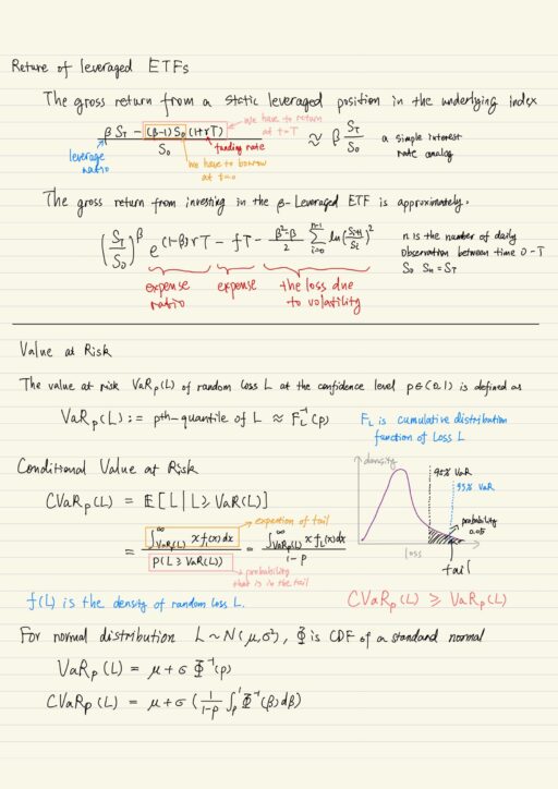
Value at Risk and Conditional Value at Risk
The value at risk VaRp(L) of random loss L at the confidence level p ∈ (0,1) is defined as p-th quantile of the loss. VaR is a tail risk measure, increasing in p, so VaR0.99(L) >= VaR0.95(L).
Conditional value at risk CVaRp of random variable L is the expected loss beyond the value at risk level. You compute the conditional probability of the loss beyond VaR, and take expectation according to it. CVaR is also a tail measure, CVaR >= VaR, increasing in p. CVaR is also called Tail Conditional Expectation or Expected Shortfall.
VaR and CVaR for normal distribution variable is completely defined by mean μ and volatility σ.
One of the reason that VaR and CVaR is popular is because you don’t have to make distributional assumptions. As long as you have access to samples of underlying distribution, you can compute VaR and CVaR of these samples.
Value at Risk is mandated risk measure in may regulations. For some return distributions, you will get a relatively small value of VaR (which makes you think the return is better) but a larger value of CVaR. This is the reason why we are moving from VaR and going to CVaR. VaR is only sensitive to the probability of losses, meanwhile CVaR is sensitive to both the probability of losses and the location of losses.
| Pros | Cons | |
| VaR | 1. captures tail behavior of portfolio losses 2. can be robustly estimated from data (not very susceptible to outliers) | 1. only sensitive to p-th quantile (not distribution beyond) 2. incentive for ‘tail stuffing’ 3. not sub-additive, diversification can increase VaR. |
| CVaR | 1. captures tail behavior of portfolio losses beyond p-th quantile 2. sub-addictive: diversification reduces CVaR 3. Mean-CVaR portfolio selection can be solved very efficiently | 1. CVaR is defined in terms of expectation, which is sensitive to outliers. |
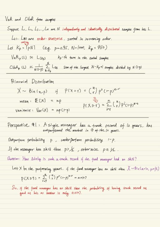
Statistical Bias
The prior hypothesis decides what kind of question is appropriate.
Average Return
Investors cars about returns to their dollars, they are caring more about a dollar weighted return. In financial market, expected returns often decrease as dollars invested increase. This is because liquidity of a market or capacity of a trading strategy is not unbounded. Small investors do not move the market. The large investors do move the market.
The more you trade in some of these markets, especially for big investors, the more you move the market against you. So you tend to see decreasing returns to dollars invested.
Average number of children in a family
What you should be doing is sampling by family. It is wrong to sample by person and getting a larger result. The bias is that it is more likely to sample children from larger family, which will over report themselves. Particularly family with zero children will be never sampled. So it is clear our bias is upwards.
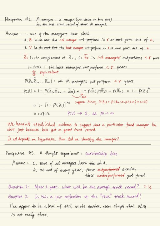
Survivorship Bias
Survivorship bias crops up an awful lot in finance and not always as obviously as we’ve seen. It needs to be born in mind by investors, risk managers and so on.
For example: stock investment. Historical returns data in the past can not be representative of the future performance. Picking stocks today and back-testing bylooking at their historical returns data is equivalent to choosing those stocks (in the past) by implicitly looking into the future. We actually introduced enormous amount of bias into our back-test. This is also equivalent to today going into the future, picking the stock in the future and trading those stock today.
Data Snooping
Data snooping arises in many context not just in finance but beyond finance and it is quite subtle and hard to spot.
For example: a bank uses historical returns data to develop a trading strategy. It first normalized the entire return data, and split them 75% as training set, and 25% as test set. The test set verified the trading strategy “is” a great success, but it actually performs poorly.
The test set should be completely unpolluted, but the test set was in the overall normalization scheme. The big mistake was we normalized the entire return data set (both training and test). Test set should have nothing to do with the trading strategy. It should have been kept entirely separate from the entire process of finding the trading strategy. What we should have done is just normalize the training set.
My Certificate
For more on Financial Engineering: Implementing Mean-Variance, please refer to the wonderful course here https://www.coursera.org/learn/financial-engineering-2
Related Quick Recap
I am Kesler Zhu, thank you for visiting my website. Checkout more course reviews at https://KZHU.ai