Assets & Portfolios: Mean-Variance Optimization

Tweet

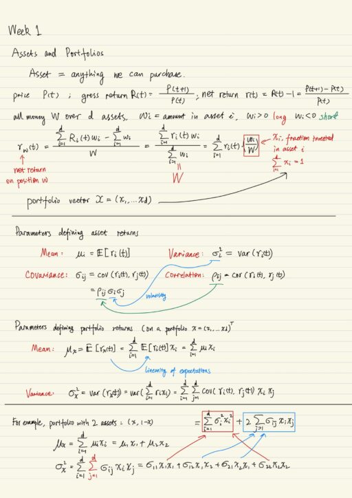
Assets and Portfolios

I’ve got a certain amount of money, I want to split it among various assets available for investment. An asset can be characterized by price and return, both of them are random. w_i is the amount of money in asset i; w_i > 0 means long investment, w_i < 0 means short investment. x_i = w_i / W is the fraction invested in asset i. What is important for the net return, is not the absolute amount of money invested, but the fraction of the total that is invested in a particular asset. So instead of worrying positions, we have to consider portfolio vector x_i. The way we deal with randomness is the quantification of mean, variance, covariance and correlation.

---

---

Diversification

Diversification reduces uncertainty. In a contrived market, assume all d assets are identical, so all of them have the same expected return μ, same volatility σ, and correlation between the assets ρ = 0. By diversifying between identical assets, we are able to reduce volatility a lot. The mean-variance portfolio selection in the end generalize this idea.

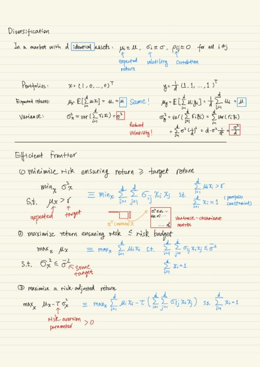
Efficient Frontier

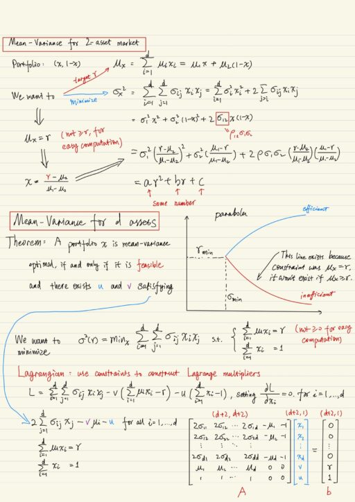
Markowitz proposed that the “return” of a portfolio is the expected return of that portfolio, and “risk” of a portfolio is to be the volatility of that portfolio. Investors would want to increase the return and decrease their risk. To calculate Efficient Frontier, we pick a particular value of volatility, or risk, and try to compute the largest return that you can get on a portfolio that has a risk no larger than a particular bound. All feasible portfolio must lie below the efficient frontier. All the space above efficient frontier is unachievable. So I only want portfolio that lie on the frontier (given a risk, maximize the return). Portfolios that lie on this efficient frontier are optimal portfolios. There are 3 different ways to compute efficient frontier:

1. minimize risk ensuring return >= target return
2. maximize return ensuring risk <= risk budget
3. maximize a risk-adjusted return

In fact, computing optimal portfolio is quite easy if there are only 2 assets; if you have any number of assets, we can form a Lagrangian using the objective function, and then convert the constrains , and multiply the them using Lagrangian multipliers and put them into the Lagrangian. At this moment, the original optimal portfolio selection problem becomes an unconstrained problem. To solve the unconstrained optimization problem, we have to compute its gradient and set it equal to 0.

---

---

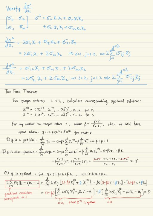
Two Fund Theorem

All efficient portfolio can be constructed by diversifying between any 2 efficient portfolios or mutual funds with different expected returns. But there are still lots of mutual funds in the market is because we are assuming all of the investors estimate the same expected return μ and the same covariance matrix σ in the future. But this assumption is never going to be true. So although is theorem is very interesting and important, there is a gap between the theory and the reality.

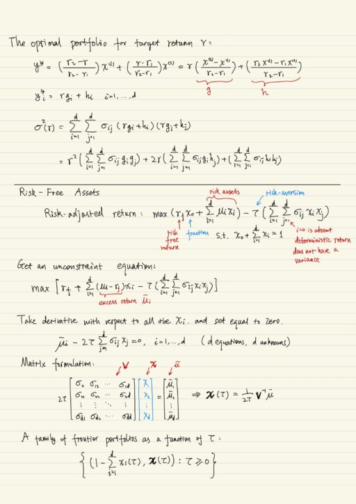
Efficient Frontier with Risk-Free Assets

Risk-free assets deterministically pays net return r_f with no risk. The fraction invested this risk-free asset is x₀. We use the formulation of maximization of risk-adjusted return to construct the efficient frontier. The entire efficient frontier can be computed by taking different risk-aversion parameter τ (>= 0). This entire mean-variance calculation is only meaningful only when target return r is greater than r_f.

The family of frontier portfolios are as a function of τ. As you crank up all possible value for τ, you will get a family of portfolios, all of the will sit on the efficient frontier.

One Fund Theorem

The risky part of the position does not add up to 1. Using the risky position by dividing it by its sum, we can construct another new portfolio position s* whose components do add up to 1. This new portfolio s* does not depend on the risk-aversion parameter τ. Essentially what everybody is doing is taking a certain amount of money x₀ putting it into risk-free asset, and remaining amount (1-x₀) invested in s*. Everybody invested in s*.

So all efficient portfolios in the market with a risk-free asset, can be constructed by diversifying between the risk free asset and a single mutual fund s*. The efficient frontier with a risk-free asset must be tangent to the efficient frontier of risk-only asset. The portfolio s* actually maximize the angle θ (between the volatility axis and efficient frontier).

Sharpe Ratio

The Sharpe Ratio of a portfolio or an asset is the ratio of the expected excess return to the volatility. The Sharpe optimal portfolio is a portfolio that maximize the Sharpe ratio. The portfolio s* is a Sharpe optimal portfolio. Everybody in the market which has a rick-free asset, diversifies between the risk-free asset and the Sharpe optimal portfolio. The investment in various risky assets are in fixed proportion, the demand for various assets are synchrony to each other, price and return should be correlated. There should be just one quantity telling us what the returns on all the assets in the market should be, because everyone holds the same portfolio.

---

---

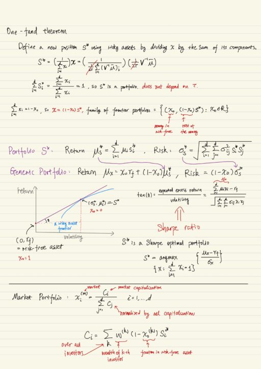
Market Portfolio

Market portfolio is defined as market capitalization normalized by the sum of all capitalizations. Suppose all investors in the market are mean-variance optimizers, then all of them invest in Sharpe optimal portfolio s*, and capitalization should completely related to Sharpe optimal portfolio. Actually the market portfolio equals the Sharpe optimal portfolio s*. The latter (Sharpe) is hard to compute, because it depends on expected return, covariance, etc; but market portfolio is much easier to compute.

Capital Asset Pricing Model

Capital market line is another name for efficient frontier with risk-free asset. It is a line goes from the risk-free asset (0, r_f) through market portfolio (σ_m, μ_m). The slope of capital market line is (μ_m – r_f) / σ_m, which is also called price of risk. Everything that is efficient must lie on this line.

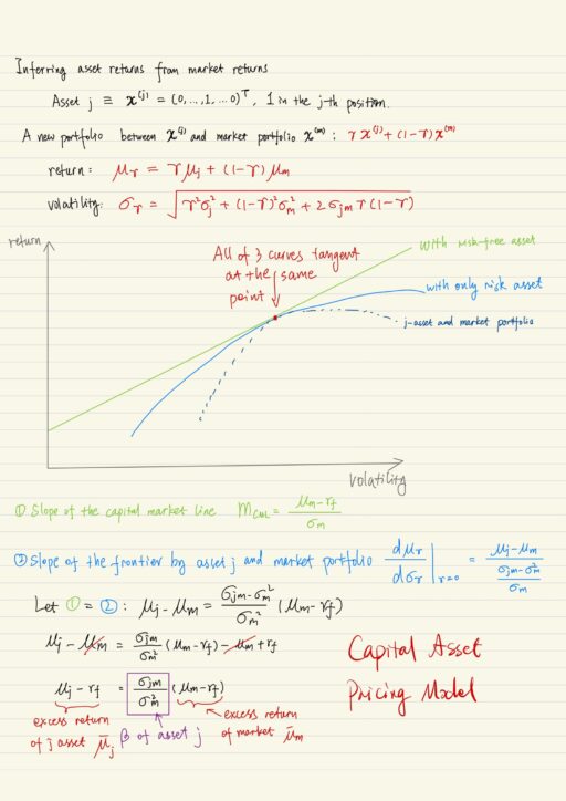
Market portfolio is there,, what we want to do is to infer asset returns from market returns. Every asset is in fact a portfolio. We could construct a new portfolio x^(γ) diversifying between the asset portfolio x^(j) and the market portfolio x^(m). We could plot 3 lines / curves together:

1. efficient frontier with risk-free asset (a line)
2. efficient frontier with only risk assets (a curve under the line above)
3. efficient frontier of the new portfolio x^(γ) (a curve under the curve above)

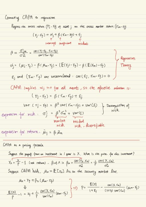
These 3 curves tangent at the same point (σ_m, μ_m), we can use this to compute what the return will be. The excess return of asset j portfolio is equal to excess return of market portfolio multiplied by β, which is covariance of asset j with market divided by the variance of market. This formulation is called Capital Asset Pricing Model. The excess return on any asset is determined by excess return on market portfolio.

In the regression of the excess return of asset j on the excess return of market. The risk contains 2 components: market risk and residual risk. But the return of asset j only depends on the market part, you don’t get compensated for residual part. This residual risk should some how be diversifiable by looking at a properly diversified asset. We should be able to get rid of it.

Security market line is another way of looking at CAPM. Plotting the historical returns of an asset with respect to the quantity r_f + β (μ_m -r_f), you should get a straight line (because they are all efficient). You should only hold those assets which are on the line or above the line.

Assumption underlying CAPM

1. All investors have identical information about uncertain returns
2. All investors are mean-variance optimizer
3. The markets are in equilibrium

Actually all of these assumptions are not true, so don’t expect all assets fall on the security market line. How to leverage deviation from security market line? There are 2 ways:

1. intercept α – hold long if positive, short otherwise
2. Sharpe ratio of a stock – hold long if > m, short otherwise

---

---

My Certificate

For more on Assets & Portfolios: Mean-Variance Optimization, please refer to the wonderful course here https://www.coursera.org/learn/financial-engineering-2

My #69 course certificate from Coursera

---

Related Quick Recap

Liquidity, Portfolio Execution, Real Options

---

I am Kesler Zhu, thank you for visiting my website. Checkout more course reviews at https://KZHU.ai

Don't forget to sign up newsletter, don't miss any chance to learn.

Or share what you've learned with friends!

Tweet