Regression and Classification Model Assessment

Table of Contents

Let’s take a look at how the performance of regression and classification models can be quantified so that we can identify the best learning algorithm to build the model. Most importantly, the learning data should be split into training data and test dtaa. Failing to hold out test data will lead to dire consequences.

Learning data: include both input features and correct answers (labels).
- Training data: for training model.
- Validation data: for hyper-parameter tuning.
- Test data: for estimating the performance of the model.

Regression Assessment

Recall that regression is about finding a function which uses some set of input features to predict some real valued number. The regression learning algorithms find that function from its hypothesis space by fitting a model to the data set. It finds the model with the least penalty according to the training data.

Once that model is chosen, we use our test data to do a valid estimate of how well the model will perform on the operational data. We test the regression model by:

Feed it the input features of test data (say X_test).
Get its best estimate of the answers in a vector (say Y^).
Measure the difference between Y^ and the correct answers (say Y_test).
We care about the magnitude of the difference:
- Mean Absolute Error (MAE): 1/n ∑ⁿ_i=1 | (Y_test)_i - Y^_i |
- Mean Squared Error (MSE): 1/n ∑ⁿ_i=1 ( (Y_test)_i - Y^_i )²
- Root Mean Squared Error (RMSE): [ 1/n ∑ⁿ_i=1 ( (Y_test)_i - Y^_i )² ]^1/2
- R-Squared (R²): 1 - [ ∑ⁿ_i=1( (Y_test)_i - Y^_i )² / ∑ⁿ_i=1( (Y_test)_i - Y_avg )² ]

A perfect model would have zero error whether it’s MSE, RMSE, or MAE, but that is also extremely suspicious.

RMSE offers better intuition than MSE about what that average error actually means, the predictions are (on average) off by that amount.

MSE is the most commonly used, but increasingly sensitive as the errors get bigger, so the model is better off making several small mistakes than a big one. MSE sacrifices perfect fit on a few data points to compensate for big mistakes, in other words, one outlier in the test data makes our model look worse under MSE than it would under MAE.

R² looks at the variation or noisiness of the model labels. R² is normalized and it lies between 0 and 1, with 1 being the best value. R² is usually used for interpretation without knowing the scale of the data and it explains how well the variation in the data itself explains the variation in the predicted values.

Different kinds of mistakes can matter more than others depending on your problem, you would want to use weighted error functions, by assigning different weights to different kinds of error. For example, penalize overestimating values twice as heavily as underestimating.

Classification Assessment

Recall that classification is about finding a model that labels data points with the correct class or category. The most common and natural way to assess a classification model is to calculate the accuracy, i.e. the percentage of correct predictions of all predictions.

Accuracy doesn’t always tell the complete story. For example:

Type 1 error: mislabeling a healthy patient as sick.
Type 2 error: mislabeling a sick patient as healthy.

The Type 2 error is much worse than the Type 1 error. and Accuracy can not directly measure both types of error. Here we need confusion matrix:

		Actual Label	Actual Label
		Healthy	Sick
Predicted Label	Healthy	True Positive (TP) (Accurate)	False Negative (FN) (Type 2 Error)
Predicted Label	Sick	False Positive (FP) (Type 1 Error)	True Negative (TN) (Accurate)

Then a few measurement defined as below:

Accuracy	Actually the true estimates `(TP + TN) / Total`
Precision	Percentage of correct positive examples of all positive examples. `TP / (TP + FP)` `Precision = 1` means we never call a patient sick inappropriately.
Recall	How much you can trust the coverage of our positive label, where TP + FN is the actual number of positive instances. `TP / (TP + FN)` `Recall = 1` means we did not miss any sick patient.
F1-Score	Balance between Precision and Recall `2 * Precision * Recall / (Precision + Recall)` `F1-Score = 1` means we have perfect Precision and Recall.

Imbalanced classes is another case where plain accuracy may not be good enough. For example: many more examples of one class (healthy individuals) than another (those with some rare disease). In the worst case, the best hypothesis will be the one that completely ignores the rare cases and just predicts the majority class. When you want to know how well classifiers performing specific to a class label, you can use class-wise accuracy.

Learning Curves

Learning curves is a set of tools that help us find the right complexity for our model and avoid overfitting. There are two key factors affect the generalization ability of a model:

Model complexity
Size of training data set

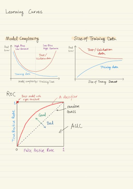
Model Complexity

Too simple	under-fitting: prediction error in both training data and test data will be high.
Too complex	over-fitting: prediction error is very low for training data, prediction error for test data will be high.

We can change the complexity of the model by altering various hyperparameters of the learning algorithm in training, for example: the degree of the polynomial features.

If we were to plot the errors on training and test data for models of different complexity, you’ll see how both errors go down up to some point. But in many cases after a certain point, the training error continues going down, but the error on test data goes up. This point is where the model starts overfitting to the training data due to excessive complexity. Stopping before test errors starts increasing would be ideal.

The same thing can happen for fixed model complexity but increasing training time, particularly in the case of neural networks where they run over that training data many, many times. As you train more and more on that same data your learning algorithm is tuning its model more and more to fit the training data. You want to stop before overfitting becomes a problem.

With validation data set, you can use learning curve to diagnose the problem. You can plot:

the performance on training data, along with
the performance on validation data

versus different model complexities or time spent in training. The performance on the validation set can act as a proxy for performance on the test data set. You stop at the correct point in complexity and the correct point in training time.

Size of Training Data

If you have more data for training, the ability of your model to generalize, almost always becomes better. If we were to plot the learning curves of the training test data for different training data set sizes for fixed model complexity:

A small training data set	Low training error, test error will be really high. Because it hasn’t learned much about the variations in the data distribution.
A large training data set	Training error increases, because the variance in training data has increased while the model complexity was fixed. Test error goes down, because the model can now generalize better.

Receiver Operating Characteristics (ROC)

ROC specifically measures the performance of classification models. For binary classification, when you have a choice of threshold, the ROC curve lets you see the trade-off between precision and recall. It illustrates the capability of the classifier to distinguish between two classes as the class discrimination threshold varies. This is achieved by plotting True Positive Rate (Recall) against False Positive Rate.

True Positive Rate = TP / (TP + FN) = Recall
False Positive Rate = FP / (FP + TN)

A point in the ROC curve represents the classification model with a specific threshold setting determining the class and the ROC curve represents the collection of such points. The best possible classification model with the right threshold setting would give a point in the upper left corner (True Positive Rate = 1, False Positive Rate = 0). This essentially means no false negatives (FN = 0) and no false positives (FP = 0). A random guest such as a fair coin flip would give a point along a diagonal line which goes from the bottom left to the top right.

Area Under the Curve (AUC) of the ROC curve represents the probability that a classification model will rank a randomly chosen positive instance higher than a randomly chosen negative one. 0 ≤ AUC ≤ 1. AUC = 0.5 means the model does not actually separate the classes.

Validation Procedures

There are two different kinds of data:

IID: independent identically distributed, and
everything else.

IID Data

IID-data is independent which means none of the data points and their labels depend on each other in a probabilistic sense; and is Identically distributed which means every data point id drawn from the same distribution.

Once we select the percentage of test data, we split our IID data randomly into train and test. But in certain cases, random splitting of the data does not work, it will end up that training data contains only 1 class. In order to solve this problem, we need stratified spit, which is when the class ratio of the learning data set is maintained in the train and test sets respectively.

Non-IID Data

Non-IID data can have dependencies for many reasons: inherently sequential (like characters in words), or distribution is changing over time (like seasons causing different pattern of snowfall). Randomly splitting non-IID data will cause problems like losing the inter-dependency which might be important. You need to either get rid of the dependency or honor them by not randomly splitting your data.

Make sure that you are dividing the data in such a way that both of training set and test set reflect different aspects of temporal data, such as seasonality and stationarity. You know what characteristics of your problem and data you have to consider when splitting up the data. Using your own knowledge about the problem domain and what you’ve learned about the actual data, you can make the right choices to ensure good clean assessments of your models.

Hyper-Parameters and Validation Data

Typically, each learning algorithm has a set of parameters (called hyper-parameters) that are not learned while training, for example:

the maximum depth of a tree
the k for k-nearest neighbors
the learning rate α for gradient descent, or
the number of hidden layers in a neural network.

These hyper-parameters are set based on the problem being solved and the domain, not just the data the learning algorithm is training on. They are different from the model parameters (such as weights) that the learning algorithm is choosing.

We want to do some decent tests to decide what combination of hyper-parameters should we have, but we can not use test data to do these tests, since test data is deserved for testing the final model. This is where the validation data comes in. We use it like the test data, but this time repeatedly to tune the hyper-parameters and evaluate which combination of hyper-parameters works the best for us.

Then once you have a model with tuned hyper-parameters, we use the test data to report the final performance as an indicator of how well our model will perform on operational data.

Cross Validation

Data is precious. Training data can be split into k segments, where each segment is used for model validation in single round and used as part of the training data in the other rounds. In the end, the average of the k validations will be reported as the cross-validation performance. Cross-validation is mainly used when the dataset is relatively small. We can reuse the data as much as we can and the result will be a good approximation of the result we would have gotten if we’d used the full dataset. This can help alleviate the problem with small datasets not being able to represent the true distribution of the data at least to some degree. We use cross-validation performance to tune for hyper-parameters in general.

Hyper-Parameter Tuning

For most of the algorithms, there are hyperparameters that have to be set by us, rather than being learned or tuned directly by the learning algorithm. For example, in neural networks, number of hidden layers, and learning rate are hyper-parameters, while weights in neuron are model parameters. Hyperparameters are determined or given before the models executed. Sometimes a hyperparameter can change during execution.

In practice, there are a couple of techniques to identify the best combinations of hyperparameters: grid search (a systematic approach) and random search.

Grid Search
- Grid search is the systematic approach. You make a list of predetermined values, usually based on covering the space of possibilities at some reasonable scale, and then simply train a model based on all possible combinations.
Random Search
- You provide a range of values for each hyperparameter of your algorithm. The system selects random values within these ranges and tries out different combinations.

Research has shown that random search actually does a better job of finding optimum parameters than grid search.

My Certificate

For more on Regression and Classification Model Assessment, please refer to the wonderful course here https://www.coursera.org/learn/machine-learning-classification-algorithms

My #94 course certificate from Coursera

Related Quick Recap

Logistic Regression & Support Vector Machines

I am Kesler Zhu, thank you for visiting my website. Check out more course reviews at https://KZHU.ai

Don't forget to sign up newsletter, don't miss any chance to learn.

Or share what you've learned with friends!