Logistic Regression & Support Vector Machines

Tweet

Often, some of the “shifts” we need to make when we’re using regression based approaches for classification. There is a major family of classification algorithms called Logistic Regression.

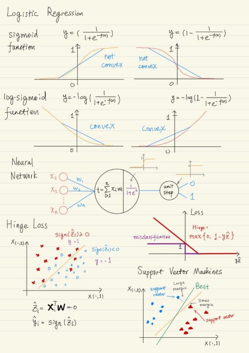
Logistic Regression

Logistic regression is actually a classification, it does not answer questions with a real number, it answers with a binary category 0 or 1. It consists of:

A regression model	The output of regression model can be thought of as the probability that a data point belongs to a particular class. If the probability is greater than a threshold, say 0.5, it belongs to class 1, otherwise class 0.
A transfer function	The logistic transfer function maps the entire real line (all rational numbers) and transforms it into a space of between 0 and 1 (something that we consider as a probability). A typical example of the transfer function is the sigmoid function.

---

---

Convexity of Transfer Functions

However, recall the definition of convexity – A convex function is a continuous function where, when you draw a line between any two points on the function, all the points on that line lie above the function. If we are using a squared loss to evaluate the parameters of our logistic function (with sigmoid transfer function), that is not convex. We can not guarantee that a bottom of a hill is actually the lowest possible point, we could get stuck in the local minimum.

To solve this convexity problem, you can actually pick a complementary loss, so that you do get a convex loss landscape called matching losses, then the minimum point is the global minimum. In the case of sigmoid function, we could use log-sigmoid function instead to get a convex and smooth landscape, and then gradient descent will help you find the optimal model.

Implement As A Neural Network

Generally speaking, neural networks are by no means limited to being used only for classification and regression. In fact, neural networks can also be found in unsupervised and reinforcement learning. Neural networks are really a sophisticated technique for function approximation, which is finding complex functions to describe the patterns you care about.

Deep learning algorithm start with a huge hypothesis space. That’s why they’re extra useful when you have lots and lots of data but can have issues with over-fitting.

A neural network is a number of interconnected neurons. A neuron is simply a function that takes some number as inputs and gives a number as output. The default way to connect them is in layers. The output of one layer of neurons serves as the input to another (feed-forward neuron networks). Typically each neuron actually involves two separate simple functions:

A linear function	Differentiable and convex, easy to calculate, but not everything fits on a line.
A nonlinear transformation / activation function	Examples: sigmoid, hyperbolic tangents, rectified linear units (ReLU), etc.

---

---

The output of the activation function is the output of that neuron, and the output of one neuron is the input to a neuron in the next deeper layer, until the final neuron outputs the final answer. The weights of the linear functions is what a neural network is learning. They are learned using gradient descent.

You could actually implement logistic regression as a neural network:

1. One input layer: for features
2. A single-neuron output layer:
   • performs the usual linear operation, and
   • transforms the output by sending it through the logistic transfer function (sigmoid function), to get a probability.
3. The probability is compared against a threshold to arrive at a class by using a unit step function.

For the last neuron, it is easy to adjust its weights to minimize the loss by comparing its output and the correct label. For each of the hidden layer, use gradient descent to iteratively adjust the weights, this is called back-propagation.

One of the open problems around neural networks is explain-ability. We currently can’t explain the choices of a neural network to a human.

Support Vector Machines

Recall the idea that using a line for classification by converting the category labels to integers. Using a line to predict the new integer class labels is not a very good idea. Looking for lines that split the space rather than fit points can work better. The classification problem can be thought of as using some kind of transfer function to convert the real numbers, to the category labels we need for classification.

Data → [Linear Regression] → Real Numbers → [Transfer Function] → some domain

Option 1: If a sign function is used as the transfer function for binary classification with the natural mis-classification loss, it will produce a flat loss surface almost everywhere. This will let us lose the ability to use iterative numerical solvers on such a loss.

---

---

Option 2: If a sigmoid function is used as the transfer function, this is just the logistic regression. Logistic regression uses the sigmoid function to convert the real numbers to probabilities as a proxy for classification. But this creates a new quandary: we could not use any loss function. We have to use a specific loss function to fix the non-convexity of sigmoid function. The combination of the loss function and the transfer function has to be a convex surrogate for our misclassification loss. This way, we can solve the classification problem effectively but in an indirect way.

Option 3: Use Hinge loss function. It is a surrogate of misclassification loss, and has some very nice properties for finding the best decision boundary for classification.

Hinge Loss Function

The best possible line would make as few classification mistakes as possible. The misclassification loss penalizes every incorrect classification. The misclassification loss is defined like this:

1. The class label is either 1 or -1.
2. Define the misclassification loss to be 0 if the real class matched, or 1 if class did not match.
   Lossmisclass = 1 if mismatch: 1 × -1 = -1, or -1 × 1 = -1
Lossmisclass = 0 if match: 1 × 1 = 1, or -1 × -1 = 1
   We treat every misclassification as equally bad.

We could impose stronger penalties for data point that are found deeper in the territory of the wrong class. The farther the misclassifications are from the decision boundary, the more wrong we are, the higher the penalty. The line or hyperplane (decision boundary) is described by the weight vector w→. For a data point, if z^ = x→⊤w→ = 0, then that data point x→ is exactly on the decision boundary, otherwise, it is on one side or the other. Also we use the sign function to determine which side of the decision boundary that particular data point falls on, i.e. y^ = sign(z^) = sign(x→⊤w→).

We introduced an extra dimension whose purpose was to divide the space into positive and negative. So in the linear part of our function, the data points further from the decision boundary will be mapped to a increasingly positive or increasingly negative numbers depending on which side of the line they’re on. The value z^ is exactly the notion for a signed distance from the decision boundary. We can use it to create a penalty that’s magnified by distance from the linear separator. How far from the decision boundary is defined as y * z^, where y is the correct label.

• y * z^ < 0: data point is on the wrong side of the decision boundary.
• y * z^ ≥ 0: data point is on the right side of the decision boundary.

We want to penalize nearly wrong classification, create some margin for error around the decision boundary. We typically give ourselves a margin of 1. We want to penalize placing the line less than one unit away from a point even if it’s correctly classified. The value of 1 - y * z^ will be positive for any points that encroaches on that margin or is incorrectly classified by our line. This way, not only will incorrectly classified points get penalties, but correctly classified points that are in that margin space around the line will also receive small penalties.

However, if we used 1 - y * z^ as our loss, the correctly classified points would get a negative penalty which is wrong. We can fix it by filtering losses less than zero. This brings us to the final formula for hinge loss:

Losshinge = max{0, 1 - y * z^}

The hinge loss is actually a pretty good surrogate for misclassification loss and it’s convex.

---

---

Objective Function

When doing classification, the optimal decision boundary is as far as possible from all of the data points. In other words, the best decision boundary maximizes the distance (known as margin) between itself and the closest data points from both classes. More precisely, in the case where the data is linearly separable and we don’t allow any mis-classification, it’s the decision boundary that’s the same distance from the closest points from both classes. Since Support Vector Machines are trying to maximize the distance (margin), they are also called Large Margin Classifiers.

These data points which are closest to the best decision boundary are called support vectors.

Linear Regression	1. Find the weights that minimize the loss. 2. Use regularizers to control complexity.
Support Vector Machine	1. Find the weights that minimize the aggregate hinge loss. 2. Use L2 norm as weight regularizer, ensuring the minimum margins are being maximized. Minimum margin = 2 / ||w||2 So, minimizing the L2 norm squared regularizer causes maximum minimum margin.

The formulation of SVM objective function is:

argminw,b C * Losshinge + regularizer
⟹ argminw,b C * [ ∑ni=1 max{0, 1 - yi * z^} ] + ||w||2
⟹ argminw,b C * [ ∑ni=1 max{0, 1 - yi * (w→⊤x→ + b)} ] + w→⊤w→

C is a smoothing parameter that controls the trade-off between model complexity and accuracy:

C → ∞	Hard margin SVM, which works only on linearly separable data. Force all hinge losses to be exactly zero.
Small value for C	Soft margin SVM. The smaller the C used, the more the algorithm will prefer to put data points on the wrong side of the decision boundary, if it keeps the norm of the weight vector down, causing a bigger margin among the data points that are on the correct side, but also likely increasing the generalization power, at least up to some point.

If your data is linearly separable and you use a very high value for C, minimizing the SVM objective function finds exactly the line that gives you the widest minimum margin possible. This is due to:

1. You are penalizing anything that has a margin less than one, because of the triangle on the positive side of graph of hinge loss, i.e. max{0, 1 - y * z^}.
2. You can change the magnitude of the w vector without affecting the direction of the line.
3. You’re pushing w to be as small as possible with the regularizer added.

If your data is not linearly separable, its penalizing misclassifications more and more as they show up deeper and deeper on the wrong side of our decision boundary.

---

---

When to Choose SVMs

SVMs actually handle nonlinear relationships rather well. Because SVMs are based on convex optimization, you don’t need as much data as Neural Networks do, to have confidence that you have found the best model in the hypothesis space.

Predicting with an SVM model is quick, especially compared to kNN with large datasets or deep neural networks. They do require homogenous appropriately scaled features. If you have mixtures of features, such as categorical and numeric, you probably want to consider decision trees or random forests.

Kernels

First, let us recall how linear regression create a non-linear decision boundary:

• By adding or transforming your features into some non-linear version of the original, you move your data into new space, which consists of nonlinear functions.
• Then in this new space, you find a linear separator (just like linear regression) with nonlinear features, where you found the line to fit the new nonlinear space.
• Transform back to the original space of features, the linear separator found in the new space will be a nonlinear decision boundary in the original space.

SVMs give us the ability to use nonlinear features in a very convenient way. The L2 norm ||w||2 in the SVM objective function also gives us the Representer Theorem.

When you use an L2 regularizer, the best weight w is for sure a weighted combination of the training data points.
w→* = ∑ni=1 αi yi x→i

Representer Theorem

This is because if you moved away from that to something that’s not entirely a weighted combination of the training points, you would strictly increase the regularizer while causing no change in the hinge loss. The Representer theorem, rather than solving the problem in the space of features and finding the best line there., allows us to:

1. Solve the problem in another space (the dual space), get a solution.
2. From the solution in dual space, recover the solution in our original space of features.

With the Representer theorem, this dual space happens to be just the space of similarities to data points. In other words, instead of finding a line that sits the space of feature values, we find the line in the space where each axis or new feature is a degree of similarity to a certain data point in the training data.

Original space	n data points, m dimensional
Dual space	n dimensional space of similarities to each of the n training data points

In the dual space of similarities, you’re not restricted to similarity in the original space. You can calculate the similarity between two points in a space other than the original feature space. For example, in the case of Polynomial Feature Expansions. Instead of looking at similarity between two data points in the original space, we can calculate similarity in the Polynomial Expansion of the feature space. For many transformations, calculating that similarity is calculating a simple function with two points as inputs. This similarities are called kernel functions.

This gives you the ability to easily use nonlinear features, gives us more complex models which is very useful if we use wisely. You can do feature expansions that expand the features into an infinite-dimensional space, which is not possible if we’re using an explicit nonlinear feature transformation.

---

---

My Certificate

For more on Logistic Regression & Support Vector Machines, please refer to the wonderful course here https://www.coursera.org/learn/machine-learning-classification-algorithms

My #94 course certificate from Coursera

---

Related Quick Recap

Linear Regression

---

I am Kesler Zhu, thank you for visiting my website. Check out more course reviews at https://KZHU.ai

Don't forget to sign up newsletter, don't miss any chance to learn.

Or share what you've learned with friends!

Tweet