The purpose of fitting models to data is to help answer research questions. We specify models based on theory or subject matter knowledge and then we fit these models to the data that we’ve collected, assuming that the variables in our dataset follow distributions or have certain relationships. The models that we fit to the datasets describe those distributions or describe the relationships. Moreover, we may be interested in predictions and want to characterize prediction uncertainty.
Types of Variables
We need to think carefully about the types of variables that we’ve collected when summarizing data:
| Categorical variables | Take on small number of discrete values (either ordered or not) |
| Continuous variables | Take on many possible values usually related to a distribution |
Another important classification of variables is the dichotomy between dependent variables and independent variables:
| Dependent variables (DVs) | Outcome, response, endogenous variables or just variables of interest. We want to specify a model to model distributional features for dependent variables, possibly as a function of other predictors or independent variables. |
| Independent variables (IVs) | Predictor variables, covariances, regressors, or exogeneous variables. These are the variables that are being used to predict the values on the dependent variables of interest. |
When we fit models to data, we examine the distributions of dependent variables that we’re interested in, conditional on the values of the independent variables, that’s our objective. And our research question defines what the dependent variable is and what the independent variables are. This involves:
- selecting reasonable distribution for the dependent variable (e.g. normal distribution).
- defining parameters of that distribution (e.g. the mean) as a function of (or conditional on) the independent variables.
Independent variables are theoretically relevant predictors of dependent variables. We are interested in estimating the relationships of independent variables with dependent variables.
Independent variables may be manipulated by an investigator in randomized experiments (in this case we have a little bit more power to make causal inference), or could simply be observed in observational studies (in this case, we only want to describe the relationship, it is hard to make causal inference about the relationships).
- If IVs are continuous, we can estimate functional relationships of those IVs with distributional features of the DVs.
- If IVs are categorical, we can compare groups defined by the categories in terms of distributions on the DVs. Avoid estimating functional relationships of categorical IVs with DVs, since actual values of categorical IVs may not have any numerical meaning.
Control Variables
Remember, our goal is to estimate parameters that describe the relationships of independent variables with dependent variables.
| In randomized study designs | We attempt to ensure randomized groups (say, a treatment group and a control group) are balanced with respect to other “confounding” variables that may have negative impact on estimation of relationships of group with DVs. |
| In non-randomzied (observational) designs | The groups that define the independent variable may not be balanced. So, randomization is a tool that we can use in study design to make sure that the values on all other variables of interest that may be related to the dependent variable are equivalent between the two randomized groups (say, treatment and control), and we lose this control when we talk about observational designs. |
When fitting models, we can include several independent variables to effectively adjust for the confounding problem. These variables are called control variables.
For instance, if we’re interested in comparing the distribution of blood pressure (dependent variable) between males and females, and we know based on our subject matter knowledge that weight is related to blood pressure, we could include weight in our fitted model as a control variable.
The weight is just another independent variable, but we can control for the value of it when talking about the relationship between gender and blood pressure. Given the inclusion of this control variable in the model, we can make inference about the gender and blood pressure relationship, given a value of weight (so as to conditioning on a value for weight). That’s the idea of including these control variables to adjust for confounding.
Missing Data
Before we start fitting models to data It’s very important that we conduct simple descriptive and bivariate analyses of the distributions on the dependent variables and independent variables, and check for missing data on both the dependent variables and the independent variables.
Listwise deletion is where units of analysis will be dropped from the analysis, if there is any missing data on any of the independent variables or dependent variables. If the units of analysis dropped due to missing data is systematically different in some way from the data but are ultimately analyzed when fitting the model, we could be introducing bias in the estimates of our relationships, and certainly, we don’t want to do that.
Implications of Study Designs
The overall idea here is that different study designs generate different types of data, and this has implications for the models that we fit to data. It’s critically important to understand how the data were generated. The data may be generated
- From a carefully designed probability sample (featuring clustered sample)
- From a convenience sample (non-probability sample)
- From a longitudinal study
- From a simple random sample
- From a natural / organic process
One key aspect of estimating the distributions of variables of interest is the possibility that different values on a dependent variable of interest may be correlated with each other. Often times, different types of study designs can introduce those correlations between different values on the same dependent variable. This may be a feature of the data that we need to account for when specifying our models.
Simple Random Sample
Take simple random sample (SRS) as an example. SRS generally produce observations on variable of interest that are independent and identically distributed (i.i.d) from carefully defined populations. When fitting models to data from SRS, we select distributions for variables with important property that all observations in data are independent (i.e. unrelated to each other).
A nice feature of simple random sampling is that, because all these observations are independent, we ultimately have more unique statistical information, which leads to the smaller our standard error is going to be, and the sampling distribution’s going to shrink. That means for us is that we have more precise estimates.
Clustered Sample
Another example is the clustered sample, which arise from study designs that generate clusters of related observations. Because observations from same naturally occurring cluster will tend to be similar to each other, we need to account for this correlation when fitting model to data (unlike models for SRS).
When we think about the standard error of an estimated mean, that standard error would reflect this correlation. Because some of our observations are correlated with each other, we don’t have as much independent information as we would have in a simple random sample. This leads to a higher standard error, and more variability in sampling distribution depending on what clusters are ultimately sampled for the study.
Longitudinal Study
Another common study design is longitudinal study. In longitudinal data, we collect repeated measures of the same variable, collected from the same unit over time, and these observations are likely correlated with each other. So models that we fit to repeatedly-measured variables in longitudinal studies need to account for this within-unit correlation.
Objectives of Fitting Models
We have two main objectives when we want to fit statistical models to data:
- Making inference about the relationships between the variables in a given dataset
- Making predictions or forecasting future outcomes based on models that were estimated using historical data
Making Inference
Independent variables are seen as a potential predictor of the dependent variable (i.e. the variable of interests). Suppose the predictor is x, and dependent variable is y. The regression function is defined as:
y = a + b x + c x2 + e

where
a: mean y when x is equal to the overall mean x in the dataset
b: expected rate of increase in y when standardized x is 0
c: non-linear acceleration in y as function of x
e: error ~ N(0, σ2)
If our objective is to make inference about the relationship between x and y, we’re interested in estimating of the regression parameters a, b, and c, and calculating the standard error. Then we can
- test hypotheses about whether parameters are equal to zero (if that parameter is zero, it is not important)
- form confidence intervals for these parameters, and determine whether or not the value of zero is contained within the confidence interval, to make inference about whether the predictor
xis important.
Recall for each parameter a, b, and c, we could calculate a test statistic t = (estimate - 0) / standard error, to test the null hypothesis H0: parameter = 0. If t is large enough, they null hypothesis will be rejected and we can conclude this is a significant result, the parameter won’t be zero.
So, for each parameter a, b, and c that test statistic which represents a large distance from the null hypotheses, would suggest that the null hypothesis that the parameter is zero would be strongly rejected. We would conclude here or infer that the relationship between x and y is in fact significant.
If these parameters are no different from zero, when looking at those test statistics, we would infer that x does not have a relationship with y.
Making Predictions
After the regression function is fitted, we have got values for a, b, and c:
y = a + b x + c x2 + ewe could plug in values of x to compute predictions of y. The prediction represents expectation of what mean y will be for a future observation. However these predictions will all have uncertainty (variance). The poorer the fitted model, the higher the uncertainty (coming with high standard error).
Today visualization of uncertainty is often as important than the prediction. Always make sure to plot the uncertainty in your graph. Be hesitant to use a model with high uncertainty to make predictions until you get more data.
We can determine most of uncertainty using standard error, which provides how far we expect our estimates to deviate from the truth.
My Certificate
For more on Fitting Parametric Models to Data, please refer to the wonderful course here https://www.coursera.org/learn/fitting-statistical-models-data-python
Related Quick Recap
I am Kesler Zhu, thank you for visiting my website. Check out more course reviews at https://KZHU.ai


