As of now, it is still unclear whether it is possible to create a so-called quantum computer, a special device which will be able to perform a special set of algorithms on the application of quantum mechanical effects.
Qubit Implementation
A qubit is the smallest element for storing and processing information in a quantum computer. A qubit has two orthogonal basis states, which are denoted as |0⟩ and |1⟩. In the general case, the qubit state is a superposition of the basis states: |ψ⟩ = α |0⟩ + β |1⟩, where α and β are complex numbers. The square of each of these coefficients (α or β) corresponds to the probability of measuring the qubit as a correspondent basis state (|0⟩ or |1⟩).
In order to implement a qubit, the physical system must meet certain requirements or criteria.
Di Vincenzo criteria
- A quantum physical system on which a qubit is realized must have two distinguished orthogonal (basis) quantum states.
- It is possible to prepare a physical system in one of these two quantum states.
- There is a procedure for measuring qubit (macroscopic distinguishability of the basis states).
- One can create a universal set of quantum logic elements (gates) for the qubit.
- The decoherence time longer than the operating time of quantum logic elements.
Scalabilty is also required, it should be possible to Crete many qubits, that could efficiently interact with each other in a controlled manner, and would be protected from the influence of decoherence.
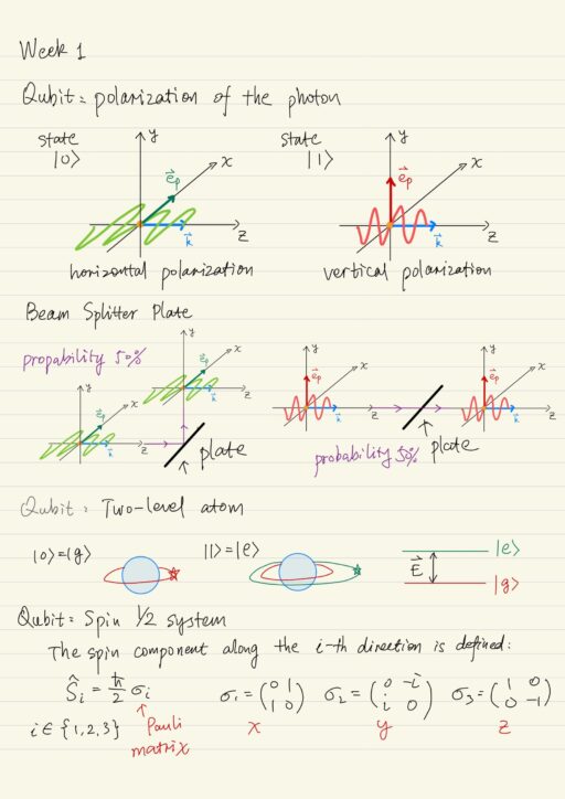
Qubit implementation: Polarization of the photon
The simplest implementation of a qubit can be carried out on the basis of the polarization of a photon. For example one basis state |1⟩ can be associated with vertical polarization, and the other basis state |0⟩ is associated with horizontal polarization. Both states are macroscopically distinguishable and can be easily distinguished using a beam splitter plate, which is sensitive to the polarization of the photon.
Other polarization direction for a photon, say circular or elliptical polarization, can be represented as a superposition of basis states corresponding to the vertical and horizontal polarization. In addition the photon is relatively stable with respect to the noisy environment that is it has great decoherence time.
However this method also has limitations:
- difficult to prepare a pulse of light which contains only one photon.
- more difficult to prepare such single-photon pulses at certain specific point in time.
- the preparing time will increase exponentially
- difficult to force photons to interact with each other
Qubit implementation: Two-level atom
Another simple implementation of a qubit is on the basis of a two-level atom. The ground state |g⟩ and excited state |e⟩ are served as the basis states of the qubit. The qubit can be performed using all the same electromagnetic waves, in principle any single qubit operation can be performed with good accuracy. For carrying out 2-qubit operations, the atoms are transferred to a state in which they could feel each others’ fields.
A common limitation is when transferring atom into special sensitive states, not only the sensitive to the filed of another atom increases but also increases the sensitivity to the whole environment.
Qubit implementation: Spin 1/2 system
Another qubit implementation is based on a particle with spin 1/2 system. Spin is a quantum physical quantity characterizing the intrinsic moment of elementary particles. Spin can also refer to the intrinsic moment of atoms, nuclei of atoms, molecules and other composite particles. The spin component along the i-th direction is defined by an operator which actually can be described using Pauli matrix.
Qubits as a rule are implemented on atoms, however it will be more convenient for us to consider an electron that also has spin 1/2 and whose spin state are clearly distinguishable, as shown in Stern-Gerlach experiment. In fact the realization of qubits on spins is simply a special case of implementation using atoms, since in the atoms the value of spin projection turns out to be associated with certain atomic levels.
Qubit as a Unit of Information
In classical computation, the unit of measurement of the amount of information is bit. If a certain physical object can take only one of two possible values, then a bit of information is required to describe such an object. If it can take m possible values, then its description requires log2m bits. The information capacity of a bit is 2N, using N bits.
A qubit in quantum computing is a unit of the amount of information. Like classical bit, it has two basis states, denoted as |0⟩ and |1⟩. However a qubit can also exist in a superposition of basis states: |ψ⟩ = α |0⟩ + β |1⟩, where α and β are complex numbers.
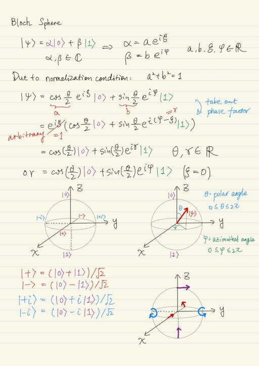
Bloch Sphere
To set the state of a qubit, we only need two real numbers: polar angle θ and azimuthal angle φ. They form a vector, running along the surface of a sphere of unit radius, called Bloch Sphere.
| positive direction coincides with | negative direction coincides with | |
| x axis | |+⟩ = (|0⟩+|1⟩)/√2 | |-⟩ = (|0⟩-|1⟩)/√2 |
| y axis | |+i⟩ = (|0⟩+i|1⟩)/√2 | |-i⟩ = (|0⟩-i|1⟩)/√2 |
| z axis | |0⟩(θ = 0) | |1⟩(θ = π) |
Each of the axes of the Bloch Sphere has a physical interpretation related to the nature of the system under consideration. In the case when qubit is realized using polarization of a photon, the Bloch sphere is called Poincare Sphere. The axes of the coordinate system are associated with the various types of polarization of photons.
Each pair of values of θ and φ corresponds to some directions of the ψ vector that are some quantum states of the qubit. The number of different states, in which one qubit can exist, is infinite. With one qubit, we will be able to encode any letter of any existing alphabet. The potential of the qubit for storing information is not limited.
However in practice we can distinguish only two states of the qubit, if we measure the qubit in the basis state |0⟩ and |1⟩, we will get qubit in state |0⟩ with probability cos2(θ/2), and in state |1⟩ with probability sin2(θ/2). The reduction of wavefunction during measurement allow us to obtain only a bit of information from the qubit state.
If the physical system is closed, its evolution occurs in a unitary way. Measurements over an ensemble of quits in the same quantum state make it possible to know this state. Quantum superposition and entanglement are critical aspects of quantum computation.
Pure and Mixed States
The pure state of a quantum system is described using a ket vector (or a bra vector), which is an element of the Hilbert space. The superposition |ψ⟩ = c1 |ψ1⟩ + c2 |ψ2⟩ + ... + cN |ψN⟩ of pure states |ψi⟩ is also a pure state. If the system is a state |ψ⟩ which is a superposition of states |ψi⟩, then it exists simultaneously in each of these states. The square of the probability amplitude |ci|2 determines the probability with which the physical system goes from the superposition |ψ⟩ to the state |ψi⟩.
A mixed state is a statistical ensemble of pure states: a system is in a state |φk⟩ with a classical probability ωk, and ∑ωk = 1.
To describe a physical system in a mixed state, one can use the statistical operator / density matrix:
ρ^ = ∑ni=1 ωi|φi⟩⟨φi|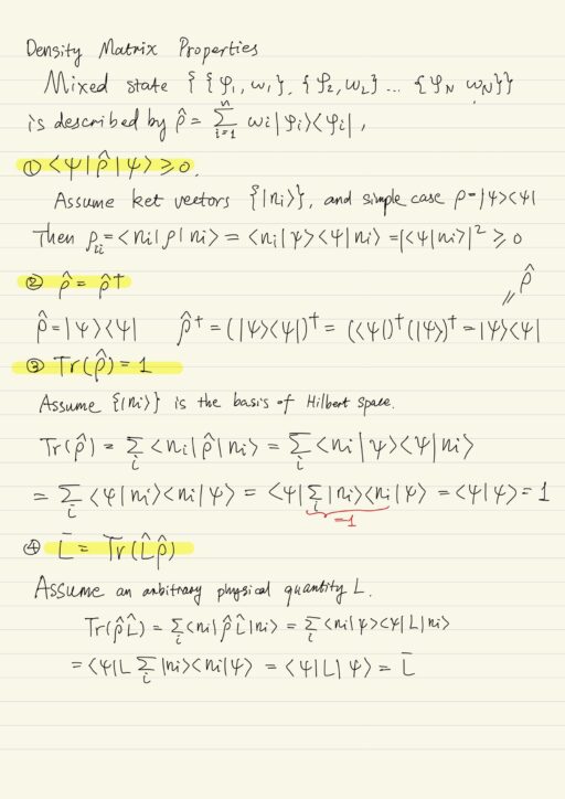
Density matrix properties
- Positive definiteness:
⟨ψ|ρ^|ψ⟩ ≥ 0for any|ψ⟩ - The density matrix is a self-adjoint operator:
ρ^ = ρ^† - Since
∑ωk = 1, the trace of the density matrix is equal to 1:Tr(ρ^) = 1. - The average of the observed L could be calculated by the formula:
L- = Tr(L^ρ^).
These properties hold when |φi⟩ form an orthonormal basis for some Hilbert space of dimension n. They also hold in general case when |φi⟩ are neither basis nor orthogonal to each other.
If a closed quantum system is in a mixed state and is described by a density matrix ρ^, then its evolution is described using the Liouvill quantum equation (von Neumann equation):
ih ∂ρ^/∂t = [H^, ρ^]Inseparability of Quantum Systems
In practice it is often necessary to deal with several interacting quantum systems, or with the quantum system consisting of several subsystems. The implementation of quantum computations requires a physical system consisting of a large number of qubits. In this case we must consider the quantum state of such a system taking into account the quantum states of each of its parts.
Suppose we have a physical system that consists of two qubits |ψ⟩ and |φ⟩ , each of which is of a subsystem. |ψ⟩ is an element of 2-dimensional Hilbert space H1, and |φ⟩ is an element of another 2-dimensional Hilbert space H2. Then the whole system will be describe as a tensor product of both vectors, which is already an element of 4-dimensional Hilbert space.
H4 = H21 ⨂ H22| Hilbert space | Basis |
| H21 | {|ψ1⟩, |ψ2⟩} |
| H22 | {|φ1⟩, |φ2⟩} |
| H4 | {|ψi⟩⨂|φj⟩}2i,j=1or {|ψiφj⟩}2i,j=1 |
For each qubit, an operator will act on the Hilbert space of this quiet and will in no way act on other qubits. For example, let the operators A^1, A^2, A^3 act on the qubit #1, and the operators B^1, B^2 act on the qubit #2, before performing the operation of tensor product, we must first find the explicit form of the operators action on every qubit, only then find the tensor product of the state vectors of all system.
A^1 A^2 A^3 B^1 B^2 = A^ ⨂ B^
where A^ = A^1 A^2 A^3, B^ = B^1 B^2
Tensor product is associative and anticommutativity.
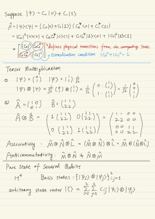
Pure states of several qubits
Consider a physical system that consists of two qubits, the basis of such a system is expressed in terms of tensor product of the basis states of each qubit. An arbitrary state vector can be represented as:
|ζ⟩ = ∑i ∑j cij |ψi⟩⨂|φj⟩If the decomposition coefficients can be chosen as |ζ⟩ = |ζ1⟩ ⨂ |ζ2⟩, where |ζ1⟩ is the state vector of H21, and |ζ2⟩ is the state vector of H22, then this state is called separable. Otherwise the state is called inseparable (or entangled).
Mixed states of several qubits
The mixed state described by ρ^ is separable if the density matrix of the entire system can be represented as:
ρ^ = ∑k ωk ρ^k1 ⨂ ρ^k2where {ρ^k1} and {ρ^k2} are mixed states for H21 and H22, and ωk ≥ 0, ∑ ωk = 1.
Otherwise the mixed state is inseparable (or entangled).
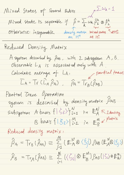
Reduced Density Matrix
It is necessary to go from the description of the whole system to the description of some parts of it. Such transition can be accomplished by averaging the density matrix of the entire system over all possible states of all its parts, except the one we want to consider.
If the physical system consists of two subsystems A and B, and is described by a density matrix ρ^AB, then to calculate the average for the observable LA (associated only with subsystem A), you can use the reduced density matrix ρ^AB:
L-A = Tr(L^A ρ^A)The reduced density matrix ρ^A can be obtained by averaging over all states of subsystem B: ρ^A = TrB(ρ^AB).
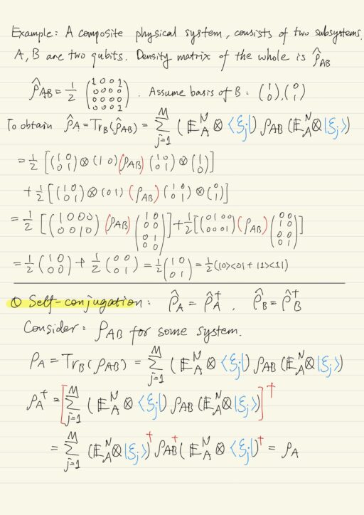
Properties of reduced density matrices
| Self-conjugation | ρ^A = ρ^†A, ρ^B = ρ^†B |
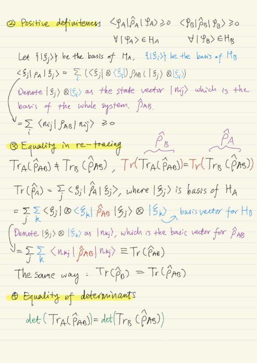
| Positive definiteness | ⟨φA|ρ^A|φA⟩ ≥ 0, ⟨φB|ρ^B|φB⟩ ≥ 0 ∀ |φA⟩ ∈ HA, ∀ |φB⟩ ∈ HB |
| Equality in re-tracing | TrA(ρ^AB) ≠ TrB(ρ^AB) However, Tr( TrA(ρ^AB) ) = Tr( TrB(ρ^AB) ) |
| Equality of determinants | det( TrA(ρ^AB) ) = det( TrB(ρ^AB) ) |
Physical system and its environment
Physical system A and its environment B form a composite physical system A + B. We can not say anything about the quantum state of system B, because it is in fact the rest of the world which consists of a huge number of the most diverse physical objects.
Separability of states
If system A and B are in a separable state, the physical system that make up the composite system are not related to each other. Both system do not interact with each other or are all isolated. Taking partial trace of entire system ρ^AB will not lose any information about the state of the system A.
If system A and B are non-separable (or entangled), when taking partial trace on the basis states of one part (say the system B), will lose information about the other one (say the system A).
My Certificate
For more on Statistical Aspects of Quantum Mechanics, please refer to the wonderful course here https://www.coursera.org/learn/physical-basis-quantum-computing
Related Quick Recap
I am Kesler Zhu, thank you for visiting my website. Check out more course reviews at https://KZHU.ai