Classification Basics
Machine learning uses learning data and learning algorithms to produce a model (or Question Answering Machine, QuAM), which is used to make prediction on unseen data. Classifier is a specific kind of model, which is built by using the supervised learning technique called classification.
Scientific method could be broken down into several steps:
- Ask a question.
- Research. See what is known and gather data.
- Develop an hypothesis. Hypothesis is a specific statement about how you thing things are, or how they work.
- Experiment and analyze the data.
- If data supports the hypothesis -> new theory.
- If not, hypothesis is rejected or modified -> Go back to step 3.
We choose to trust those hypotheses that match experimentation and data analysis, and call them scientific theories. We then use these scientific theories to predict new phenomenon.
Supervised learning is learning from correctly labeled examples. Supervised learning can be compared to scientific method.
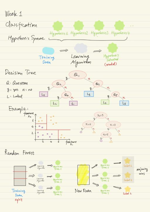
- Ask a question. There might be many hypotheses (in the hypothesis space) that answer the question, but most of them are incorrect. For classification, the hypothesis space includes any function that categorizes the data into classes.
- Research. Training phrase (fitting a model to the data) to filter out bad hypotheses.
- Feed training data into a learning algorithm
- The learning algorithm evaluates different hypotheses by testing their ability to predict the categories in the training data and throws out those that do a bad job.
- The learning algorithm selects a single model or hypothesis that best fits the data it has.
- That model can be used in the inference or prediction phase where we use the operational data.
There are several ways we narrow down the hypothesis space. For classification, we only care about hypotheses that actually predict class labels.
Decision Trees
If we want to build a classification model, each example in our learning data will have to be labeled with their appropriate classes. These labels form an unordered set of classes.
The decision tree works by constructing a series of yes-or-no questions. A good example is a binary tree. In each of the node, a question is asked with an yes-or-no answer. We follow the path and continue to ask yes-or-no questions until we reach an endpoint (a leaf). That leaf tells us which class that example belongs to.
Decision trees are a type of classifier that split the space based on a sequence of binary choices with respect to a single feature. The main idea is to find a feature and a split point within that feature splitting the data set into separate classes. The actual results highly depend on the learning algorithms, e.g.: some use information theory, some use statistical techniques, etc.
In a more complex and realistic situation, when to stop is also critical. Complete seperation sounds nice but it is actually not great, because it results in over-fitting. The model is not going to generalize well to unseen data.
Decision trees are easier to interpret than other models. They can also handle multi-class classification when working with more than just two binary classes. On the other hand, they tend to be unstable: any little variation in training data might result in a totally different decision tree.
Ensemble Learning, which combines several models to try to improve predictive performance, is a way to mitigate the instability. For decision trees specifically, an ensemble method is known as Random Forest. One disadvantage however is that it is obviously slower than a single decision tree. It is also more difficult to interpret a forest than a single decision tree.
Generalization and Overfitting
Machine learning can be described as the process of generalizing from data. The generalization is limited by two things:
- The example your model has to learn from.
- The learning algorithm you use to train your model.
To test the generalization capabilities of your model, you need to test it on unseen data. The learning data is split into training data and test data.
| Training data | The labeled data to train the model on. |
| Test data | The labeled data to evaluate how well that model generalizes to unseen data. Compare the labels the model predicts to the labels we already have. |
Overfitting can be thought about as your model fitting to irrelevant details. We don’t want our model to memorize exactly the examples at scene because it is not going to generalize well to new data. Over-fitting occurs when our model is too complex given the size of our training data, probably because of the number of features, or the complexity of learning algorithm we choose to use.
Underfitting is when our model is not complex enough to capture meaningful nuances, that are relevant to new unseen data, in our data. So we want to model in between these two things: fitting training data well enough, and still generalizing well to new unseen data.
When it comes to decision trees, the main idea behind all techniques is that “smaller trees mean less overfitting”. These usually can be specified as parameters in function calls:
| max leaf nodes | Upper bound on how many leaves are allowed in the tree. |
| min samples per leaf | Minimum number of examples that must end up at each leaf. |
| max depth | The depth of the tree (the total number of decisions) |
We can also prune some of branches of a tree to take away some of the detail. Pruning usually uses cross-validation or validation scores to identify which portions of the tree can be pruned.
| Pre-pruning (early stopping) | Pruning done while building the trees Faster, but there are chances that it could underfit the data, as it just give an estimate of when it should stop. |
| Post-pruning | Pruning after the decision trees have been built. Not based on an estimate, but actual values. |
k-Nearest Neighbours
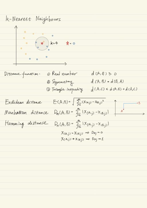
kNN is one of the simplest machine learning algorithms, its essence is comparison. The kNN QuAM predicts what category a new example belongs to by figuring out which of the stored examples are most similar (nearest neighbours). It checks what category those neighbours belong to, and make an educated guess that this example belongs to the same category as the majority of its neighbours.
Each of examples is represented by the computer as a list of number (the feature vector), similarity between two feature vectors can be measured by a distance function. If we have training data set which is represented by an m-by-n matrix (m examples, n features), to classify a new example, the model need to carry out 3 steps:
- Compute the distance between the new example and every other example in training set.
- Pick the k closest neighbours.
- Conduct a majority vote. Whichever label gets the most votes from those neighbours, is the class for the new example.
Unlike most other classification methods, kNN is a type of lazy learning, which means there is no separate training phase before classification. This highlight one big downside of this algorithm – we have to keep the entire training data in memory. So kNN usually works fine on smaller data sets that don’t have too many features.
Important decisions must be made before building a QuAM classfier based on kNN:
- the value of k.
- the distance measures.
Value of k
You may choose arbitrarily or come up with optimal value using cross-validation. It is necessary to try several different values with different QuAMs. Anyway it must lead to clear majority between classes.
The value k can also be treated as a smoothing parameter: a small value of k will lead to large variance in prediction; a large value of k means you don’t get very customized answer (large bias).
The KNN method can also be used for regression tasks, the prediction though is done through average the k most similar data points.
Distance measures
Thanks to Pythagoras theorem, we know that the squared value of the hypotenuse is equal to the sum of the squared values of the two other edges. In linear algebra, it is called the magnitude of the difference vector between two points. In fact this generalizes to m-dimensional space. We call it Euclidean distance.
Mathematically speaking, a distance function maps two elements to some real number. There are there rules that must hold for valid distance measures.
- Only positive numbers, we don’t care about direction, only distance.
- Order does not matter. Symmetry.
- Triangle inequality
A few widely used distance metrics:
- Euclidean distance / L2 norm. (Norm is the technical term for the magnitude of a vector).
- Manhattan distance / L1 norm.
- Hamming distance (for categorical or non-continuous variables).
My Certificate
For more on Classification: Decision Trees and k-Nearest Neighbours, please refer to the wonderful course here https://www.coursera.org/learn/machine-learning-classification-algorithms
Related Quick Recap
I am Kesler Zhu, thank you for visiting my website. Check out more course reviews at https://KZHU.ai