Time Evolution of Quantum States

Tweet

Time-dependent Schrödinger Equation

Time-dependent Schrödinger equations is not an eigenvalue equation, but allowing us to predict the state at t, given the initial condition at t_0.

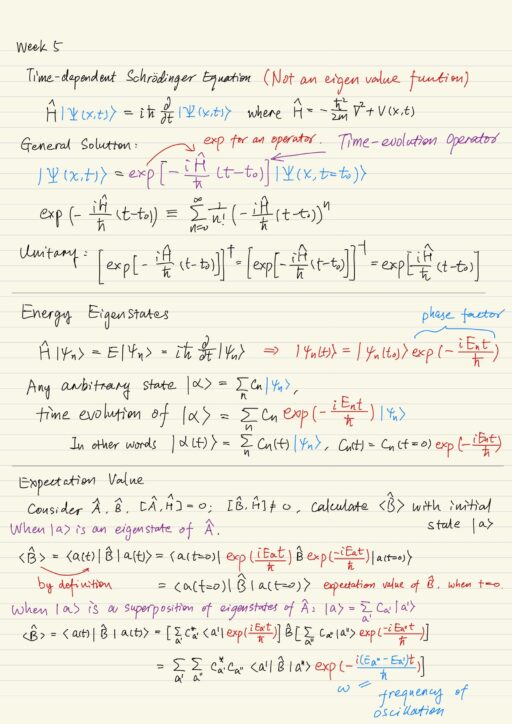
H^ |Ψ(x, t)⟩ = i h ∂/∂t |Ψ(x, t)⟩

where Hamiltonian H^ = -h2/2m ∇2 + V(x, t). The potential energy V(x, t) in general depends on time, however time-independent potential V(x) covers a large number of important problems.

---

---

The general solution can be obtained:

|Ψ(x, t)⟩ = exp[ -i H^/h (t-t0) ] |Ψ(x, t = t0)⟩

where exp[ -i H^/h (t-t0) ] is called time-evolution operator, which is unitary. Consider energy eigenstates H^ |ψn⟩ = E |ψn⟩, the solution is expressed as:

|ψn(t)⟩ = exp( -i En/h t) |ψn(t0)⟩

Constant of motion

Any arbitrary state |α⟩ could be expressed as |α(t)⟩ = ∑n cn(t) |ψn⟩ where cn(t) = cn(t=0) exp(-i En/h t). Note that the time evolution of energy eigenstates is given simply by a phase factor, and quantum state does not change (called constant of motion). This must be true for any eigenstates of an operator that commute with the Hamiltonian operator, since commuting operators share the same eigenkets (eigenstates).

If we can find a complete set of an operator that commute with Hamiltonian, then we can express an arbitrary initial state, as a linear superposition of these eigenstates in the complete set. And time evolution of this arbitrary initial state is then expressed by multiplying a phase factor exp(-i En/h t) to each of the eigenstate in the superposition.

Similar to momentum conservation in classic physics, in quantum mechanics, the similar situation would be a problem where momentum operators commute with Hamiltonian. Then the momentum eigenstates will be eigenstates of Hamiltonian as well, the time evolution of the momentum eigenstates can be described by multiplication of this simple phase factor. This equivalent to momentum conservation in classical physics.

Expectation value

Consider A^, which commutes with Hamiltonian: [A^, H^] = 0 and B^, which does not commute with Hamiltonian: [B^, H^] ≠ 0. Then the expectation value of B^ with initial state |a⟩ is like this:

|a⟩ is an eigenstate of A^	⟨B^⟩ = ⟨ a(t=0) | B^ | a(t=0) ⟩ The expectation value of B^ does not change over time (stationary), because the ket |a⟩ itself is a stationary state.
|a⟩ is a superposition of eigenstates of A^ |a⟩ = ∑a' ca'|a'⟩	⟨B^⟩ = ∑a' ∑a" c*a' ca" ⟨a'| B^ |a"⟩ exp(-i (Ea" - Ea')/h t) The expectation value will change over time with a frequency of oscillation: ω = (Ea" - Ea')/h

Schrödinger vs Heisenberg Pictures

When changing basis of state vectors, the unitary operators only change their representation. and do not actually change the state vectors / kets. But there are also unitary operators that actually change the state kets, for example: translation, rotation, and time evolution.

Let’s denote the evolution operator (unitary) as U^, and then the time evolution of a state |α⟩ can be written as |α⟩ → U^ |α⟩. Note that unitary transformation preserves the inner product ⟨β|α⟩ → ⟨β| U^{^†} U^{^} |α⟩ = ⟨β|α⟩.

The time evolution of matrix representation for operator X^ can be interpreted in two but equivalent ways:

⟨β| X^ |α⟩ → ⟨β| U^† X^ U^ |α⟩
= ( ⟨β| U^† ) X^ ( U^ |α⟩ )
= ⟨β| ( U^† X^ U^ ) |α⟩

Schrödinger picture	the operator X^ is time-independent while state kets evolve over time as described by U^ |α⟩ and ⟨β| U^†.
Heisenberg picture	the state kets remain time independent while the operator varies over time as U^† X^ U^.

In classical physics, we do not use state kets and only deal with time evolution of observables, thus Heisenberg picture could provide a closer connection with classical physics.

We can explicitly write the state kets and observables in Schrödinger and Heisenberg pictures. Recall that the evolution operator is U^ = exp(-i H^/h t), assuming t₀ = 0, then the operator A^{^} in Heisenberg picture may be written as the operator A^{^} in Schrödinger picture, or vice versa:

A^(H) = U^† A^(S) U^
A^(S) = U^ A^(H) U^†

Similarly for state kets:

|α⟩(H) = |α(t=0)⟩(S)
|α⟩(S) = U^|α⟩(H)

Expectation value remain the same in both pictures:

(S)⟨α(t)|A^(S)|α(t)⟩(S) = (H)⟨α(t)|A^(H)|α(t)⟩(H)

Time evolution of an operator A^{^} in Heisenberg picture (Heisenberg’s equation of motion):

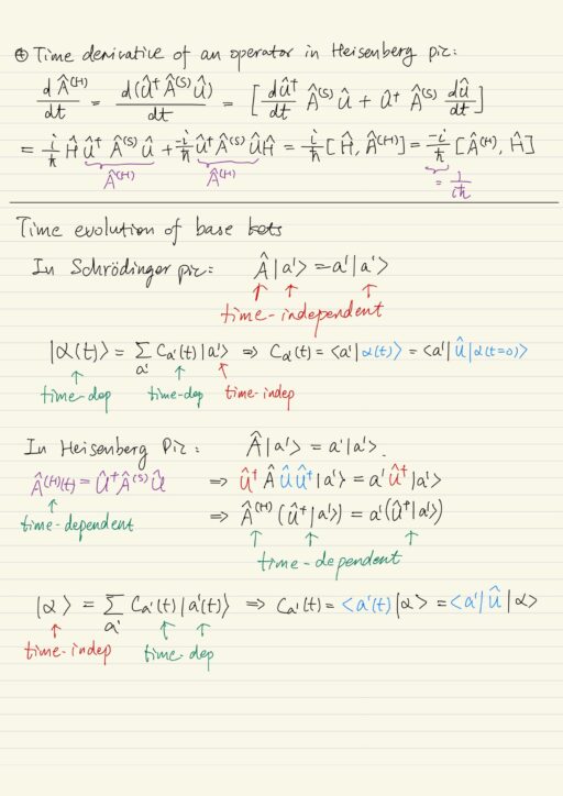
dA^(H)/dt = (1/ih) [A^(H), H^]

Whereas the time evolution of state kets in Schrödinger picture (Schrödinger’s time-dependent equation):

H^ |Ψ(x, t)⟩ = i h ∂/∂t |Ψ(x, t)⟩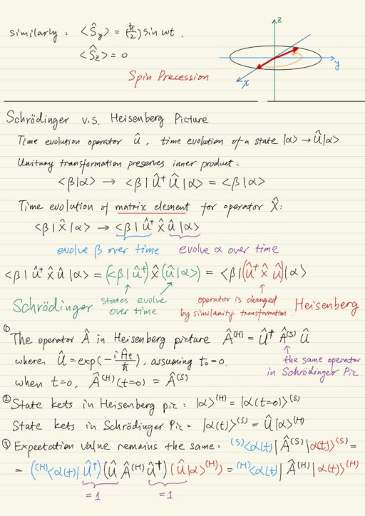

---

---

Time evolution of base kets

In Heisenberg picture, the base kets (the kets used as basis) are time-dependent. Because they are also the eigenkets of an Hermitian operator, which is time-dependent in Heisenberg picture. However the state kets in Heisenberg picture are time-independent. Recall state kets are used to describe a quantum state and are superposition of base kets.

In Schrodinger picture, the base kets are time-independent. Because the operators are time-independent, therefore their eigenkets should be time-independent.

Expansion coefficients are however the same in both pictures.

	Operator	State kets	Expansion Coeff	Base kets
Heisenberg Picture A^(H) (U^†|a'⟩) = a' (U^†|a'⟩) |α⟩ = ∑a' Ca'(t) |a'(t)⟩	A^(H) time-dependent	|α⟩ time-independent	Ca'(t) time-dependent	|a'(t)⟩ time-dependent
Schrödinger Picture Heisenberg Picture A^ |a'⟩ = a' |a'⟩ |α(t)⟩ = ∑a' Ca'(t) |a'⟩	A^ time-independent	|α(t)⟩ time-dependent	Ca'(t) time-dependent	|a'⟩ time-independent

Harmonic Oscillator

Let us reconstruct the eigenstates of harmonic oscillator using annihilation and creation operator instead of solving Schrödinger’s time-independent equation.

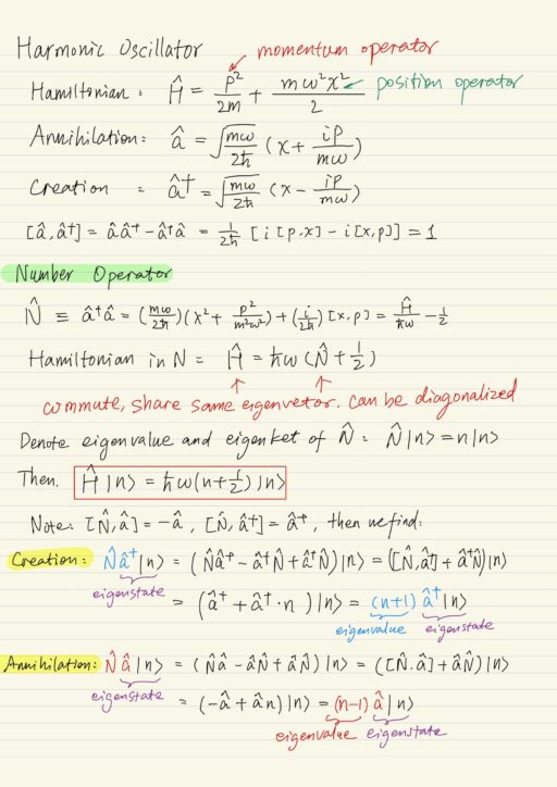
For simple harmonic oscillator, the Hamiltonian is here, where p and x are momentum operator and position operator respectively.

H^ = p2/2m + (1/2) m ω2 x2

We also define annihilation and creation operators, which do not commute [a^, a^†] = 1.

a^ = √(m ω / 2h) (x + ip/mω)
a^† = √(m ω / 2h) (x + ip/mω)

Number operator and states

We could define the number operator as N^ = a^†a^ = H^ / hω - 1/2, then the Hamiltonian written as:

H^ = h ω (N^ + 1/2)

H^{^} and N^{^} commute, share the same eigenvectors, and both can be diagonalized simultaneously. Denote the eigenvalue and eigenket of N^{^} as N^ |n⟩ = n |n⟩. Then it follows that:

H^ |n⟩ = h ω (n + 1/2) |n⟩

The eigenstate of N^ (represented by |n⟩) is called the number states. They are also eigenstates of H^ with energy eigenvalue of En = h ω (n + 1/2).

Creation an Annihilation operators

Note the commutation relation [N^, a^] = -a^ and [N^, a^†] = a^†. Then the states a^{^†}|a⟩ and a^{^}|a⟩ are also eigenstates of number operator N^{^} with eigenvalues raised or lowered by 1, which mean creating one quantum or decrease one quantum, respectively.

Creation:     N^ a^† |n⟩ = (n+1) a^† |n⟩
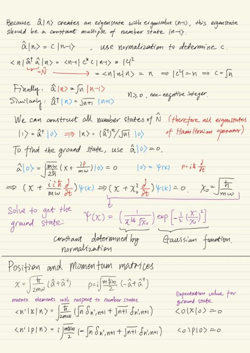
Annihilation: N^ a^ |n⟩ = (n-1) a^ |n⟩

Because the annihilation operator a^ operating on the number state |n⟩ creates an eigenstate with an eigenvalue (n-1), this state should be a constant multiple of number state |n-1⟩.

a^ |n⟩ = √n |n-1⟩
a^† |n⟩ = √(n+1) |n+1⟩

The minimum allowed value of n is zero, we can construct all number states, and therefore all eigenstates of Hamiltonian operator.

|1⟩ = a^† |0⟩
|n⟩ = (a^†)n/√(n!) |0⟩

By solving the equation a^ |0⟩ = 0, we could find the ground state |0⟩, i.e. the lowest state ψ(x) using position representation, and then we successively apply the creation operator to this function ψ(x), and then we generate all wave functions of harmonic oscillator problem.

---

---

Position and Momentum matrices

The position and momentum operators can be represented in terms of creation and annihilation operators.

x = √(h/2mω) (a^ + a^†)
p = i √(mhω/2) (-a^ + a^†)

The expectation value for the ground state are both zero.

⟨0|x|0⟩ = 0
⟨0|p|0⟩ = 0

The expected value of x2 and p2 operator for the ground state:

⟨0|x2|0⟩ = h/2mω
⟨0|p2|0⟩ = hmω/2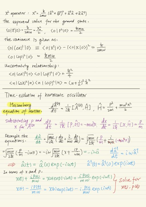

TIme Evolution of Harmonic Oscillator

Here we are going to solve Heisenberg’s equation of motion in order to discuss the time evolution of harmonic oscillator states. We use Heisenberg’s equation of motion and Hamiltonian, and substitute p and x:

dp/dt = -mω2x
dx/dt = p/m

We need to use annihilation and creation operators to decouple them, finally solve for x(t), and p(t):

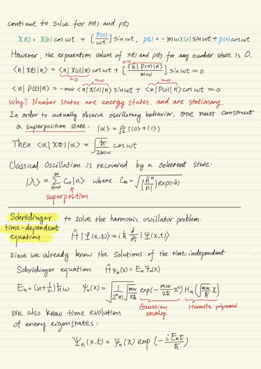
x(t) = x(0) cosωt + [p(0)/ωt] sinωt
p(t) = -mω x(0) sinωt + p(0) cosωt

However, the expectation value of x(t) and p(t) for any number state |n⟩ is zero, because number states are energy states, and are stationary. In order to actually observe oscillator behavior, we must constructa superposition state. Classical oscillation is recovered by a coherent state.

We can also solve the harmonic oscillator problem using the time-dependent Schrödinger equation. The resultant probability density functions are identical to the Heisenberg picture before. The difference is where the time dependence is attached – wavefunction or operator.

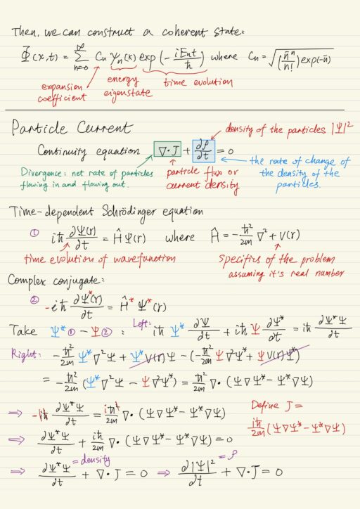
Particle current

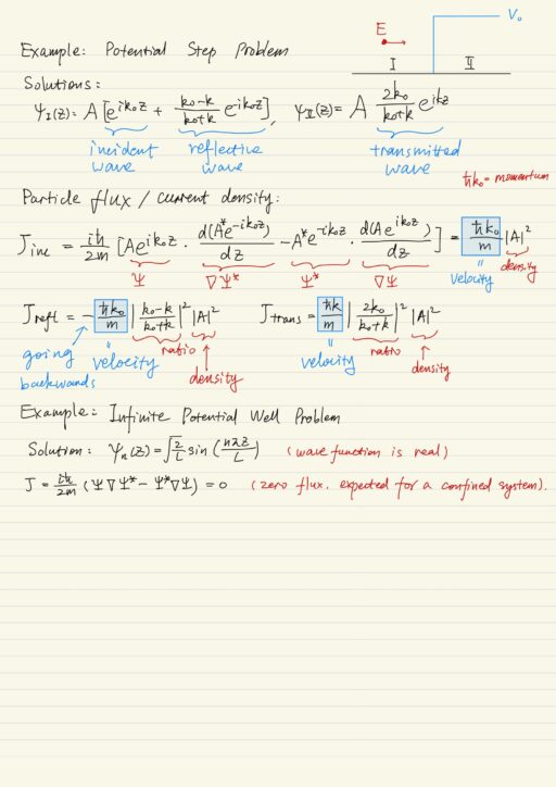
In the potential step and barrier problems, we calculated the transmission and reflection coefficients from the ratios of the probability amplitudes. This is perfectly fine if we are dealing with actual waves as in optics and acoustics. In quantum mechanics, we are dealing with particles that behave like waves.

Particle current is related the rate of change of particle density via the ‘continuity equation’, where J is the current density and ρ is the density of the particles. This equation is valid as long as there are no creation or annihilation of particles.

∇∙J + ∂ρ/∂t = 0

In quantum mechanics, particle density ρ is given by the absolute value square of the wavefunction |Ψ(r)|2, because this is basically the probability of finding a particle. J is defined as (ih/2m) (Ψ ∇Ψ* - Ψ* ∇Ψ).

---

---

My Certificate

For more on Time Evolution of Quantum States, please refer to the wonderful course here https://www.coursera.org/learn/foundations-quantum-mechanics

My #83 course certificate from Coursera

---

Related Quick Recap

Quantum Mechanics: Uncertainty Principle and Change of Basis

---

I am Kesler Zhu, thank you for visiting my website. Check out more course reviews at https://KZHU.ai

Don't forget to sign up newsletter, don't miss any chance to learn.

Or share what you've learned with friends!

Tweet