Multi-period binomial model
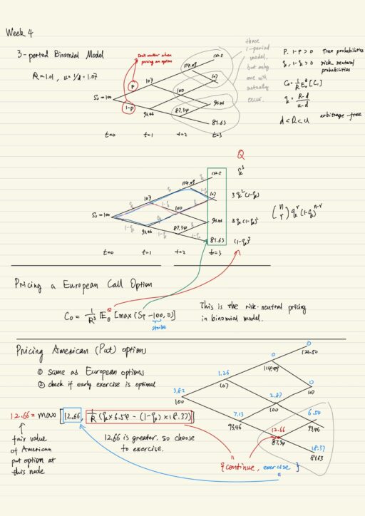
Multi-period binomial model is really just a series of one-period model spliced together. When pricing an European option, you can calculate it backward 1 period at a time. But you may also do the same thing just as one calculation.
It appears the true probabilities p (price going up) and 1-p (price going down) does not matter. Only the risk-neutral probabilities q and 1-q matter. Actually you should NOT expect to see 2 securities with extremely different true probabilities. Option pricing theory simply states that if you have 2 securities in the economy then they will have the same option price.
Another interesting observation is the gross risk-free interest rate R increased, the option price also increases. This is totally against what you would see in a deterministic world. In a deterministic world, when interest rate increased, you decrease the present value of the cash flow.
Recall our analysis of the binomial model, “no arbitrage” is equivalent to d < R < u. Any derivative security with time T payoff CT can be priced using this function C0 = (1 / Rn) * EQ0 [CT], where q > 0, 1-q > 0 and n is the number of periods. This representation is actually more general. This is first fundamental theorem of asset pricing:
- In fact for any model, if there exists a risk-neutral distribution, such that the equation holds, then arbitrage can NOT exist.
- The reverse is also true, if there is no-arbitrage, then a risk-neutral distribution exists.
Pricing American Options
We can price American options in the same way as European options, but now must also check if it is optimal to early exercise at each node. NOTE, recall that it is never optimal to early exercise an American call options on non-dividend paying stock, so consider put options.
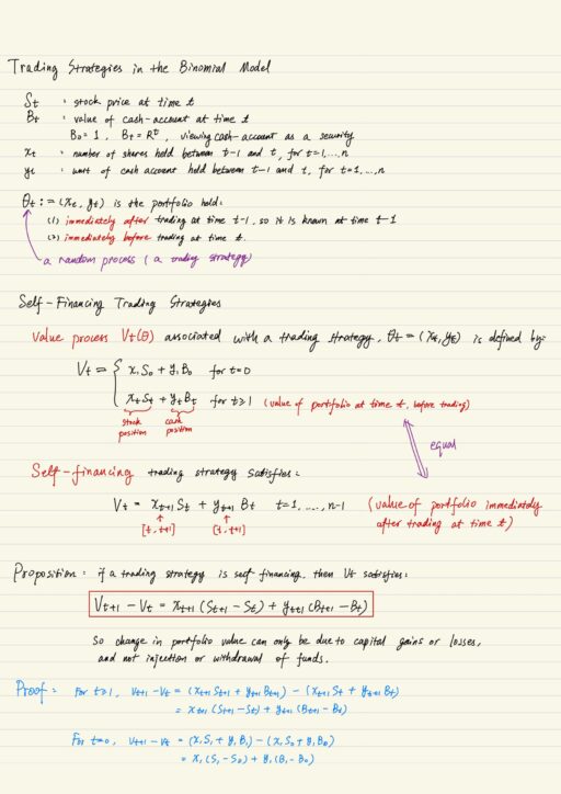
Self-Financing Trading Strategies
It is a trading strategy θt – (xt, yt) where changes in Vt are due entirely to trading gains or losses, rather than the addition or withdrawal of cash funds. The definition states that the value of a self-financing portfolio just before trading is equal to the value of the portfolio just after trading, so there is no funds have been deposited or withdrawn.
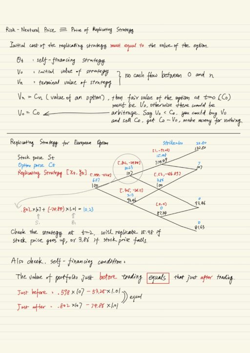
Risk-Neutral Price = Price of Replicating Strategy
Dynamic replication: you are using a trading strategy which adjusts the holdings in the stock and cash account at each time, so that at maturity we replicate the payoff of the option.
In the multi-period mode we can do the same as what we have done in single-period model. We can construct a self-financing trading strategy that replicates the payoff of the option. The initial cost of this replicating strategy must equal to the value of the option, otherwise there is an arbitrage opportunity. The dynamic replication price is of course equal to the price obtained from the risk-neutral probabilities and working backwards in the lattice. At any node, the value of the option is equal to the value of the replicating portfolio at that node.
Including Dividends
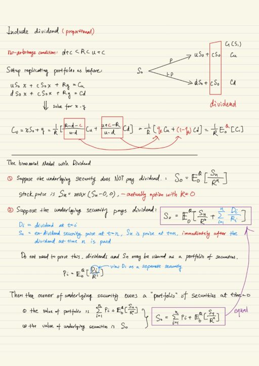
Consider again 1-period model and assume stock pays 1 proportional dividend of cS0 at t = 1. Now no-arbitrage condition is d + c < R < u + c. We can again use 1-period replicating strategy to replicate the payoff of this option. In multi-period binomial model, we can assume a proportional dividend in each period. Each embedded 1-period model has identical risk-neutral probabilities. We can view the i-th dividend as a separate security. Then the owner of underlying security owns a ‘portfolio’ of securities at time = 0.
Pricing Forwards and Futures in binomial model
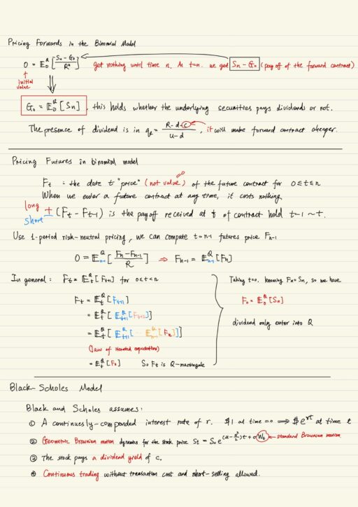
When you buy a forward contracts, no money changes hands, and in fact initial value of forward contract is zero. The so-called forward price G0 = E0Q[Sn] is used to determine the payoff at the maturity of the forward contract. If the underlying security pays the dividend, it goes into the risk-neutral probabilities Q. The presence of dividend will make the forward contract a little cheaper.
The fair value of a future contract at any time is actually zero. When price of a future contract Ft is really used to determine the payoff of owning it. Fn = Sn by definition. Ft is not how much you need to pay when buying or how much you receive when selling. A future contact always cost nothing. Ft is only used to determine the cash-flow associated with holding the contract. ±(Ft – Ft-1) is the payoff received at time t from a long (+) or short (-) position of one contract held between t-1 and t. So a future contact is always worth zero, but pays “dividend” Ft – Ft-1 at time t. The price of futures is F0 = E0Q[Sn].
The price of forward contracts and futures contacts is equal, even though they are different contracts. The futures marks to market everyday, there is ‘dividend’ payoff everyday, where as the forwards pay nothing everyday until maturity. But they actually have the same price F0 = G0. This is ONLY try in binomial model, because interest rates are deterministic and Rn can be eliminated. In general interest rates are random.
Black-Scholes Formula
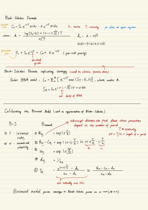
The Black-Scholes formula is of great importance in industry, and we can view the binomial model as approximation to the Black-Scholes formula. Notice the μ (drift of Geometric Brownian motion) does not appear in the Black-Scholes formula, which is similar to the p (real probability) of option pricing formulas in binomial model. Once we know the price of European call option, we can calculate the price of European put option by using put-call parity (with dividend yield c).
Industry practitioners use Black-Scholes formula to quote the price of options. Binomial model is often used as approximation to it. But one needs to calibrate the binomial model by translating Black-Scholes formula parameters into the Binomial model parameters.
Pricing a European put on future contract
Many of the most liquid options are options on futures contracts. Trading lots of stock indices are expensive and time consuming, so we don’t trade these indices, we trade futures of these indices. In practice we don’t need a model to price liquid options, actually demand and supply determine the price of options. This amounts to determining the implied volatility σ. The model helps us in two ways: first, it determines the exotic and more illiquid securities whose price are not available in the markets; second, it help hedge options.
My Certificate
For more on multi-period binomial model, please refer to the wonderful course here https://www.coursera.org/learn/financial-engineering-1
Related Quick Recap
I am Kesler Zhu, thank you for visiting. Check out all of my course reviews at https://KZHU.ai
