Exploration and Planning in Reinforcement Learning

Table of Contents

Exploration is needed to find unknown actions which lead to very large rewards. Most of the reinforcement learning algorithms share one problem: they learn by trying different actions and seeing which works better. We can use a few made-up heuristics (e.g. epsilon-greedy exploration) to mitigate the problem and speed up the learning process.

Multi-armed bandits

An Markov Decision Process with only single one step is also known as multi-armed bandit. The agent only sees one observational state, it then picks an action and get feedback (reward), then the whole session terminates. Next session (also contains only 1 step) is completely independent with the previous session.

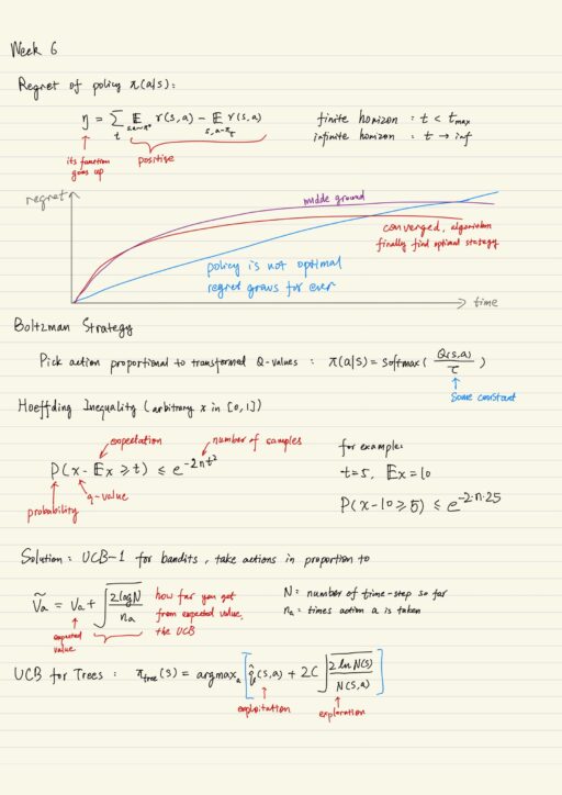
Regret

Regret is basically how much reward your algorithm wasted, or how much reward you could have earned if your algorithm used the optimal policy from the beginning.

Exploration Strategy

epsilon-greedy
- For example, value-based algorithms: Q-learning, DQN, SARSA, etc
- with probability ε, take a uniformly random action
- with probability 1-ε, take the optimal action
- the figure of regret: it will start low, but keep growing and grow linearly because the agent never finds the optimal policy. We have to decrease ε over time until it reaches zero.
Boltzmann
- pickup actions proportionally to the transformed Q-values
algorithms with built-in exploration
- cross-entropy methods, policy gradient family (REINFORCE, actor-critic)
- all explicitly learn the probability of taking actions
- affect them with regularization of entropy, but actually algorithms decide exploration policy themselves.

How do we human explore? Humans are not epsilon-greedy. The actions that are uncertain, whose outcomes are not yet well known to us. To actually implement this in practical algorithm, let us model “how certain we are” that “Q-value is what we predicted”. It is our belief expressed as probability distribution that the Q-value will turn out to be some number. Our challenge is to pick up an action, not just given the action value, but also given the belief we have about it.

Thompson Sampling

1. sample once from each Q distribution
2. take argmax over samples

Frequentist UCB

In the situation where you want to explore as much as possible, you want to learn quickly which action is the best with at least some confidence ratio. A family of exploration strategy is called ‘Upper Confidence Bound’.

1. compute XX% percentile (upper confidence bound) for each action
2. take the action with the highest confidence bound

If the percentile selected is large value, it is very like to be ‘explore’, and if the percentile is small, it is very likely to become a ‘exploit’. So this percentile becomes a parameter you can change when you need. There is a number of inequalities that bound P(x > t) < some_value. They all compute probability of some value being greater than a threshold. But you don’t want to solve for the probability, what you really want is t (the threshold).

Bayesian UCB

1. Start from prior distribution P(Q) - for example: reward in bandit setting, or Q-function in multi-step MDP setting
2. Learn posterior distribution P(Q | data) - posterior distribution of the same variable after observing some data, namely the action you have taken in some states, and the rewards you've got.
3. Take n-th percentile of the distribution learned, sort actions by percentiles, and then pick whatever you want

There are 2 main families of methods that allow us to learn the posterior distribution:

Parametric Bayesian inference
- select some kind of known probability distribution to use as P(Q | data)
  - normal distribution (franchised with mu and sigma squared)
- the problem: whole rely on the distribution
Bayesian neural network
- learn a neural model which predicts a distribution
- a neuron is not a number but a distribution
- to get the whole picture, you have to repeat the sampling procedure many times until you get enough data t calculate the percentile

Advantage
- no longer depend on inequality, instead you have a particular distribution (gives exact choice of prior)
- able to engineer a particular formulation given all the export knowledge you have about it.
Drawback
- the choice of prior may make or break (for example: over-explore, not certain of anything; or alternatively too greedy to learn the optimal policy)

Planning

Model-free setting	Model-bases settings
we know nothing about environment dynamics p(s’, r \| s, a)	we are given a model of the world, ether 1. distributional model p(s’, r \| s, a) with explicit probabilities 2. sample model (s’, r) ~ G(s, a) without explicit probabilities

What we know in model-based settings are about immediate rewards, we still don’t know global estimate of return for any action. We should ground our decision on the global rewards (for example, value or action-value functions). In reality, the brute force approach of “calculating and recording return value of each action of each state obtained by every policy” is simply not feasible, because of possible large state and action space.

These approaches to finding an optimal solution for “sequential decision making problem” in a model-based setting as fast as possible is called “planning algorithms”. By planning, we mean any process by which transforms the model of the world into a policy.

Type of planning

Model-free – learn the policy by trial and error
- any model-free algorithms can be used in a model-based setting
- used in many algorithms, especially in the ones which learns the approximate of the world from the interaction of the real world.
Model-based – plan to obtain the policy
- background planning
  - sampling from given environment model (either true or approximate)
  - learning from such samples with any model-free method
  - example: dynamic programming
- decision time planning
  - planing is performed to select optimal decision now in current state
  - commit an action only after planning is finished
  - example: heuristic search, MCTS

“The main difference between Background planning and Decision-time planning is that the latter plans to select optimal action only for the current state, whereas the former builds a policy that is good in every state.

The Decision-time planning may be much more applicable to the real world scenarios. In the real world a robot may face only subset of all possible states. So it is no point in wasting computational resources to build a good policy in all states, as the Background planning does.”

To obtain such knowledge, we enroll the local dynamics in time and accumulate the sequence of rewards in a single return. Planning algorithms differ mostly on how and when such enroll are performed.

Heuristic search

To solve a planning task as fast as possible, we should always expand only those actions, which are the good candidates to become the best ones. To give expansion in the direction of the most promising actions, we can use any functions which correlates with true returns that our policy is able to achieve. Such functions are usually called heuristic functions. Any planning method uses heuristic functions are call heuristic search.

Heuristic search is an umbrella term unifying many algorithms, with an idea of look-ahead planning guided by heuristic functions, selecting only valuable nodes/branches to expand.

In reinforcement learning, heuristic functions are value functions, but we might want to refine value functions over time. The advantages are that the resources are only focused on valuable paths, and nearest states contribute the most to the return.

But the drawback is also obvious:

(unreliable) approximate model will cause bad planning results. The look-ahead based on approximate model can spoil the learning, and turn the estimates of a reliable value function to become less precise. So remember it only makes sense to make planning in the model of the world, if more precise than the current value function estimates.
it depends on the quality of heuristic

One way to obtain heuristic is to estimate the return with Monte Carlo. We can try to use model of the world (instead of the function approximation) to estimate the value of possible continuation of leave nodes onward, if we limit the horizon of lookahead search. We can estimate the value of any state or state-action pair with Monte Carlo returns.

Estimate values with Rollout

1. while within computation budgets
    a. from state s make action a (using model of the world)
    b. follow rollout policy (Monte Carlo trajectory sampling) until episode ends
    c. obtain return G_i
2. by performing rollout many times, we obtain and output q(s, a) = means of G_i

The good point of Monte Carlo estimate is that it not need function approximation, it is sufficient to rely on only the model of the world. Each rollout is dependent on the others, which allows running in parallel on many CPU cores. However the precision of the estimate relies on the number of rollouts.

Select actions with Rollout

π(s) = argmax_a q(s, a)

Select an action that maximize the Monte Carlo value estimates (strikingly similar to Value Interation). If we want to make our policy π(s) close to be optimal, we should make our rollout policy as good as we can. But good policy may be slow, then it won’t generate enough number of rollouts, and degrade the overall performance.

Monte Carlo Tree Search

MCTS is a family of amazingly successful decision-time algorithms, viewed as a distant relatives of heuristic search. It is a planning algorithm requires much of computation time, heavily relying on Monte Carlo rollouts to estimate the value and action-value. A big advantage is that it won’t throw estimates away, but reserve some state-to-state estimates (reducing computation time). MCTS preserves to policies:

Tree policy (respect uncertainty, and determines the direction of the search)
Rollout policy (estimate the values)

Typical MCTS can be divided into 4 phrase, these phases should be repeated as much as possible to produce meaningful decisions. When the time runs out, the algorithm stops and best action for current state (the root of the tree) is selected.

selection
- the rollout starts from the root of the tree
- sends down the tree, selecting actions according to the tree policy
- once such rollout enters a leaf, expansion phase is launched
expansion
- current leaf’s adjacent state nodes (with all its actions) are added to the tree
simulation
- rollout policy takes control
backup
- when the episode ends, the return of the rollout is available
- the return is propagate back to each of the state-action pair we have visited by current rollout
- the cumulative discounted return (from that node to the end of the episode) is saved in each state and action node

Tree Policy: UCT

There are plenty of choices for tree policy. The most effective and popular one is Upper Confidence Bound for Trees (UCT). Tree policy should balance between exploration and exploitation. The most simple approach is to treat each action selection as an independent multi-armed bandit problem, which can be effectively solved by Upper Confidence Bound (UCB).

Select actions when planning is finished or interrupted

There are many possible strategies.

max – the root child with the biggest action-value estimate: action with highest q(s, a)
robust – the root child most visited: action with highest N(s, a)
max and robust – both most visited and highest value
secure – the root child with lower confidence bound

My Certificate

For more on Exploration and Planning in Reinforcement Learning, please refer to the wonderful course here https://www.coursera.org/learn/practical-rl

My #61 course certificate (with Honors) from Coursera

Reinforcement Learning: Policy Gradient Methods

I am Kesler Zhu, thank you for visiting my website. Checkout more course reviews at https://KZHU.ai

All of your support will be used for maintenance of this site and more great content. I am humbled and grateful for your generosity. Thank you!

Your generosity and kindness is overwhelming!

Don't forget to sign up newsletter, don't miss any chance to learn.

Or share what you've learned with friends!