Financial Engineering: Term Structure Models

Tweet

Fixed Income Derivatives

Fixed income markets are enormous and in fact bigger than equity markets. Fixed income derivative markets are also enormous, including:

• interest rate and bond derivatives
• credit derivatives
• mortgage backed securities
• asset backed securities

Fixed income models are inherently more complex than security models, because it needs to model evolution of entire term-structure of interest rates. One of the classic ways to get around this problem is the ‘short-rate’ r_t, the risk-free rate that applies between period t and t+1. It is what we are going to get at time t+1, if we deposit $1 in cash account at time t.

---

---

The philosophy behind fixed income derivatives pricing is really about extrapolating from liquid security prices to illiquid security prices, as follows:

1. specify risk neutral probabilities for the short-rate r_t , without referencing true probabilities of short-rate.
2. price fixed-income derivatives in the way that guarantees no-arbitrage
3. match market price of liquid securities via calibration procedure (by picking unknown parameters in the model)

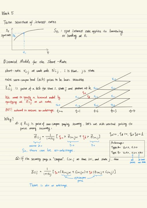
Binomial models for the short-rate

Z_i,j^k stands for the price of a zero-coupon bond for time i, state j, and mature at time k. We want to specify a binomial model by specifying all Z_i,j^k for all nodes, but it is possible but awkward to ensure no-arbitrage. Instead we use short-rate r_i,j at each node N_i,j, and Z_i,j being price of a non-coupon paying security, and then use risk-neutral pricing to price every security.

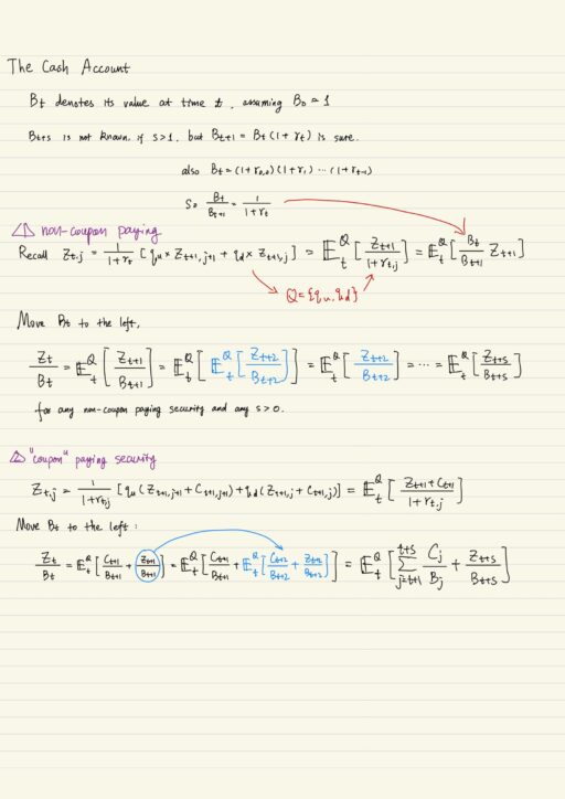
Cash Account

The cash account is a particular security that in each period it earns interest at the short-rate. B_t denotes its value at time t. Cash account is only risk-free because we not current interest rate, but not risk-free in long run, because interest rates are stochastic.

Term structure

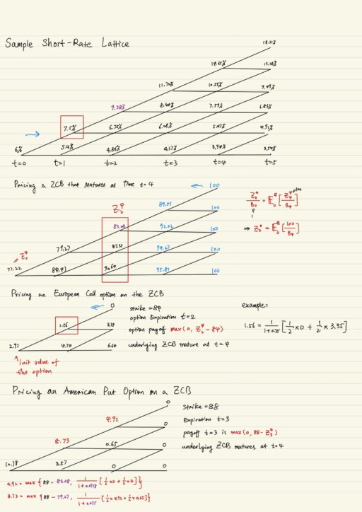
We can use risk-neutral pricing to compute the price of a zero-coupon bond. Securities that do not pay coupon or do not have intermediate cash flows, only pay its face value at maturity. Having calculated zero-coupon bond price at time t=0, we can infer from that the actual interest rate corresponding the maturity.

Therefore we can calculate all of the zero-coupon bond prices for all maturities, say: Z₀¹, Z₀², Z₀³,… then compute all corresponding interest rates s₁, s₂, s₃,… and backing them out to obtain term structure of interest rates.

Then the methods of pricing these fixed income derivatives are introduced:

1. European call and American put options on non-coupon paying bond
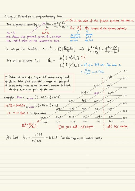
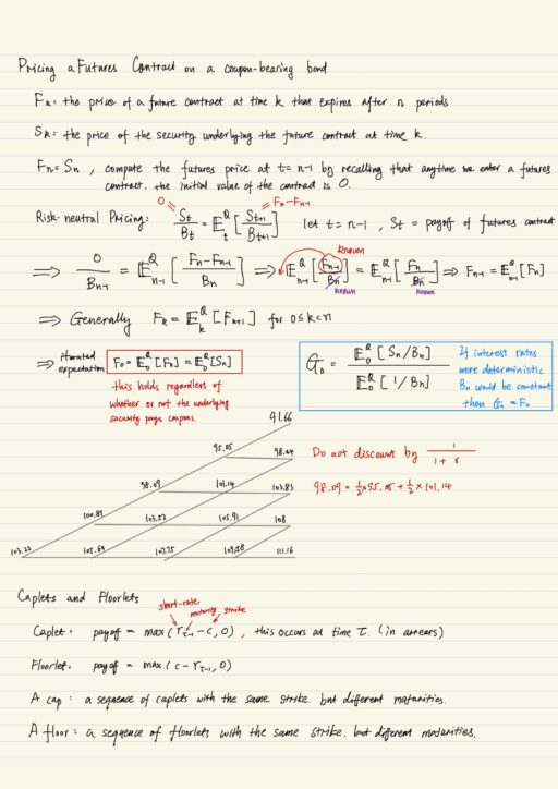
2. Forward contracts on coupon-bearing bond
3. Futures contracts on coupon-bearing bond
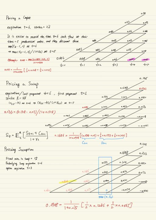
4. Caplets and Floorlets
   • Caplets and Floorlets are similar to European call option on the short-rate r_t, settled in either arrears or advance. Caps / Floors are sequences of caplets / floors with the same strike but different maturities.
5. Swaps and Swaptions
   • A swaption is an option on a swap.

---

---

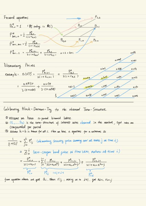
Forward Equations

Forward equations allow us to compute the price of elementary securities (Arrow Debreu securities), which pay $1 at particular time and state. Constructing forward equations will make pricing derivative securities easily. It is state price P^e_i,j denotes the time 0 price of a security that pays $1 at time j, and state j; and $0 at all other time and states.

Once we have calculated elmentary security prices using forward equations, we can use it to easily calculate the price of zero-coupon bond, and forward starting swap.

Model Calibration

How should we choose parameters of models so that model prices match the market price of liquid securities seen in the marketplace. mThere are any free-parameters, for example: r_i,j, q_i,j for all i, j.

• We can fix some parameters, say q_i,j = q = 1-q = 1/2.
• Or use parametric form, say Ho-Lee model: r_i,j = a_i + b_i * j (a_i is drift component, b_i is volatility component)

Black-Derman-Toy model assumes r_i,j = a_i e^{(b_i * j)}. Taking log of r_i,j, we have log(r_i,j) = log(a_i) + b_i * j. So drift component for log of short-rate is log(a_i) and volatility component is b_i.

We certainly want to calibrate models to zero-coupon bond prices, ideally, we also want to calibrate to prices of other securities like caplets, floors, swaptions, etc. This is done by choosing a_i and b_i to match market prices.

Pricing a Payer Swaption in a Black-Derman-Toy Model

An M-N payer swaption means an option to enter an N-year swap in M years time. Payer feature of the option means if that option is exercised, the exerciser will “pay fixed, receive floating”. Receiver option exerciser will “pay floating, receive fixed”.

Swaption prices depend on volatility (b_i). Different b_i values (even after re-calibration) will lead to different Swaption prices. The more volatile your model is or the market is, the more valuable the swaption price will be. We want to the price of the calibration securities (that is used to calibrate the model) also depend on volatility.

So if we use a model to price an exotic security, the price we get very depends on what securities I used to calibrate the model in the first place. In the lecture the zero-coupon bond is used and b_i is fixed. If a different set of securities are used (say, caplets or floorlets to calibrate the model), the we would get different result. Be careful how these models were built, and how they were calibrated.

Pricing in Practice

In practice, more complex models (than binomial models) are used to price fixed-income derivatives. However the philosophy is still the same.

1. Specify a model under risk-neutral dynamics Q(θ). θ is a vector of parameters you need to choose, like a_i and b_i in Ho-Lee or BDT.
2. Price all securities with our new model using risk-neutral pricing.
3. (Model calibration) choose θ so that market price of appropriate liquid securities agree with the model price of those securities.

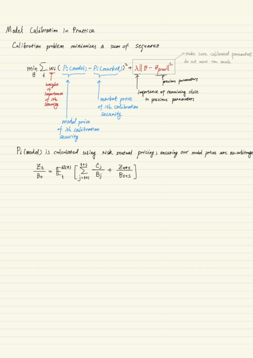
Calibration problem typically requires to selecting appropriate parameter θ to minimize the sum of squares. Once the model is calibrated, we can use it to hedge or price securities. But”

1. this model is usually very difficult to optimize, since it is usually a non-convex optimization problem with many local optima, and very hard to find the global true optimal solution.
2. as market condition changes, we need to re-calibrate frequently.
3. derivative prices and practices depend on true probabilities p and 1-p, but the dependency actually enters into the calibration process. True probabilities are reflected in the market price perceptions.

---

---

My Certificate

For more on Financial Engineering: Term Structure Models, please refer to the wonderful course here https://www.coursera.org/learn/financial-engineering-1

My #64 course certificate from Coursera

---

Related Quick Recap

Multi-Period Binomial Model

---

I am Kesler Zhu, thank you for visiting my website. Checkout more course reviews at https://KZHU.ai

Don't forget to sign up newsletter, don't miss any chance to learn.

Or share what you've learned with friends!

Tweet