Linear Regression - KZHU.ai 🚀

Table of Contents

Recall that the concept of hypothesis spaces is a collection of hypotheses that might answer a particular question, and learning algorithms find the best hypothesis in the space of functions which we’ll call the model or QuAM.

Previously we learned that classification learning algorithms operate in the space of functions that classify examples. However we can also think about hypotheses that predict numbers (regression) rather than categories (classification). The space of all arbitrary functions that return numbers is a pretty big space, one of the simplest subsets of this hypothesis space is the set of linear functions (straight lines).

Line Fitting and L2 Loss

Given a set of 2-dimensional data points, how to find the best-fit straight line? In the context of Machine Learning, this is called Linear Regression. Again, this amounts to narrowing down our hypothesis space to one particular hypothesis or model that best makes predictions on unseen data.

How to find the best line? We measure each line’s relative badness, penalize the bad ones, choose the line that has the least penalty associated with it. This penalty will be some measurement based on mistakes, the difference between value predicted and data given. We’re going to square each difference to ensure that our measurement is positive, because we don’t want our underestimates canceling out our overestimates. we only want to capture the magnitude of how far our line is from the training data.

Then the squared difference for each of our data points and then summed up to get the least squares error for the entire line. Functions that quantify this mistakes are knowns as loss functions. The best line is the one that minimizes the loss as much as possible.

training data: (x_i, y_i)
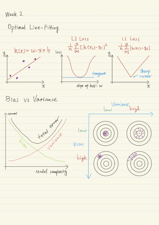
line function: h(x_i) = w * x_i + b
L2 loss function: = 1/n ∑ⁿ_i[h(x_i) - y_i]²
= 1/n ∑ⁿ_i[w * x_i + b - y_i]²

We need a strategic way to find the line that minimizes our penalty. x_i and y_i are determined by the training set, while w and b are the things the learning algorithm can adjust in its quest to find the best line. Calculus to the rescue, because loss function is both smooth and convex, which means it is going to have a unique minimum point. Using calculus can find it.

What we have is a particular total loss for each hypothesis (linear function). We can graph the total loss for each hypothesis (each particular setting for the slope w and y-intercept b). From the graph, we can see visually the minimum loss is at the lowest point of the bowl. The slope of the tangent line at a local minimum is 0, which is also the point where the derivative of the loss function is 0.

derivative of L2 loss function:
∂/∂w 1/n ∑ⁿ_i[w * x_i + b - y_i]²
= 1/n ∑ⁿ_i2x_i[w * x_i + b - y_i]
= 0

Solve for the parameters w and b, the solution definitely give us the smallest possible loss.

In fact most machine learning projects will have a very high dimensional feature space. We can do the exact same process in arbitrary m-dimensional space. Now we have a feature vector x^→, and weight vector w^→. Our goal is still to find the weight vector w^→ and b that minimizes the penalty function L2 loss.

h(x^→) = w^→⊤ x^→ + b = ∑^m_j w^→_j * x^→_j + b

We don’t even have to worry about b anymore because in general we can make one of our features a constant one and b becomes the weight on that.

L1 Loss and Convexity

We could just take the absolute value of the difference to get the actual magnitude between the predicted value and the label. This is a totally valid loss function known as the L1 loss.

L1 loss function: = 1/n ∑ⁿ_i|h(x_i) - y_i|

Just like the L2 loss function, the shape of the L1 loss is convex. It has an obvious minimum penalty value (a sharp corner). This means the function’s not smooth, and not differentiable. So we can’t use that tangent trick, take the derivative of the L1 loss to find which parameters give us the minimum penalty, like we did with the L2 loss function. We have to use some kind of iterative process: start at any odd point, then make small adjustments in our parameters to bring us closer to an approximate solution.

Across all loss functions, there’s one crucial property that each must possess if you want to guarantee you’re finding the global minimum. This property is convexity. A function is called convex, if for any two points on the graph of the function, the line segment connecting those two points lies above or on the graph. Convexity guarantees that our function has no more than one local minimum value.

So regardless of whether you use:

derivatives (if your function is differentiable), or
some other iterative numerical solver (if your function is not differentiable)

only when your function is convex, you’re guaranteed to find the optimal solution in that hypothesis space.

Iterative Method for L2 Loss: Gradient Descent

Gradient Descent is an iterative method that is very commonly used in machine learning. Iterative methods start with some initial point and then take small steps to bring us closer to an approximate solution. Because we want to minimize loss we use an iterative method by taking small steps in whatever direction the loss function is decreasing.

We care about minimizing loss functions because finding the minimum of our loss-function means finding the model that has the smallest penalty. How to use gradient descent to find the minimum of loss functions?

In gradient descent, we rely on the property that the graph is

smooth and continuous so that we can take the derivative, and
convex, so there’s no more than one minimum value.

The graph is the surface crated by the loss function over all the allowable variations of our model. We randomly pick a starting position on the graph, which means assigning random parameters to our model, i.e. an initial guess we have to start somewhere before we can improve it.

We can calculate exactly in what direction we shall move using the derivative of the slope of the tangent to the graph at this point. w_n+1 ← w_n - α ∇L(w_n), where ∇L(w_n) is the derivative with respect to w of the loss function of the current estimate, α is the learning rate or step size.

If learning rate is too big, you’ll end up stepping past local minima and you never settle on a good parameter value, i.e. diverge.
If it is too small, it will take forever to converge, to settle down near the best value.

Some techniques have decreasing alphas so that you can start big but settled right down, and depending on the rate of decrease, you can actually guarantee convergence.

Methods for L1 Loss

Like L1 loss function, there are many cases where you may have a convex function that you want to optimize but this function is not smooth at some point and so is the gradient does not exist. There are other iterative methods you can use to get close to the minimum value of the loss function, such as the simplex method.

Nonlinear Features and Model Complexity

Sometimes a linear function is not sophisticated enough to capture meaningful relationships between inputs and labels. Of course you can try to find a hypothesis in the set of things other than straight lines. But don’t forget linear features have handy features like convexity and differentiability. Luckily, we can get complexity with linear functions through feature engineering.

Polynomial Feature Expansion

One commonly used example is adding polynomial features (multiplying things together), which is called quadratic features when the order is 2. Adding or transforming features means we can have lines in the new expanded feature space that translate to things other than straight lines in the original space, even though we’re still learning a linear function. We create non-linear functions by adding or changing features that are non-linear functions of the original features, but our hypothesis space is still delightfully simple space of straight lines.

Look at any term of a polynomial in standard form and add up the exponents of that term, we get the degree of the term. The degree of the maximum degree term is called the degree of the polynomial or the order of the polynomial. For example: if we have a polynomial that has m linear features x^i₁₁ … x^i_m_m, and a term where the exponents sum up to p, i.e. i₁ + i₂ + ... + i_m = p, then our polynomial is an order p polynomial.

We call the vector of all possible polynomial combinations of our original linear feature, the polynomial feature expansion. So a feature expansion of (x₁, x₂) to degree 2 is (x₁, x₁², x₁x₂, x₂, x₂²).

Under-Fitting vs Over-Fitting

Suppose we have a bunch of points generated from an unknown relationship that has a bit of noise, linear regression model over this dataset probably won’t work because of under-fitting. To overcome under-fitting, we need to increase the complexity of the model to use a higher order polynomial equation. However keep increasing the model complexity will lead to overfitting, and a over-fitting model won’t do a good job of answering questions about data that are not in the training data set. Here test data set from the same source as the training data set, can help find the tradeoff.

Bias and Variance Tradeoff

The bias-variance tradeoff is a fundamental property of learning. In the math sense, prediction errors are either due to bias or due to variance. These two types of errors are linked, so there’s a trade-off between a model’s ability to minimize errors due to bias and its ability to minimize errors due to variance.

Bias from a particular choice of data will lead to bias from your model. But when we speak of bias of the model, we’re also talking about bias stemming from our choice of hypothesis space. The final model is biased as no choice from this space will perfectly described the real-world.

If our initial hypothesis space only includes simple models, we probably will have under-fitting, because we try to avoid over-fitting but also introducing more potential for bias. It’s unlikely the best hypothesis in this small space actually captures the real relationships.

On the other hand, if we use an excessively complicated model, which will learn noises along with signals, we will have over-fitting, and more likely our approach will have high variance. What creates the variance?

Noisy in different batches of data (even these batches are from the same source) will cause models almost always be different. A set of highly varying models will give inconsistent predictions.
Learning algorithm itself when parameters are initialized randomly. Even on the same data set, you will get drastically different models.

Bias is how far predictions are from the correct class or value, and variance is how different a model’s predictions are from each other. In the real world, we usually don’t know where the target of the model is. But still bias can be measured by looking at the performance on our learning data. Models with high bias will under-fit the training data as well as perform poorly on the test or validation data. Variance is harder to measure, but still it can be measured by looking at how much output changes when you repeat the learning process on a different sample of learning data.

Regularization is a systematic way of making the trade-off between bias and variance of your machine learning models in order to have better generalization on new unseen data. Learning curves can also be used to diagnose your model’s performance.

L2 Norm Regularizers

When a learning algorithm has an objective function that only penalizes mistakes as with the loss functions we’ve already described, we want to modify our objective function with some criteria that rewards simplicity as well as accuracy.

A regularizer is an extra mathematical term added to the objective function which penalizes complexity. Now the objective you want the learning algorithm to minimize is a combination of:

The penalty for making mistakes, as well as
The penalty for using a complex model.

The objective function would look like this, where λ acts to control the relative strength of carrying about simplicity compared to carrying about loss L.

obj function = L(w^→, X^→, y^→) + λ ||w^→||²₂

As your model gets more and more complex and more and more fitted to the training data by using higher and higher degree polynomial features, you can observe that the weights are getting larger and larger. The magnitude of weights are a good proxy to measure complexity and that’s often what we use. Regularization term will penalize extreme values for these weights.

Since we care about the magnitude and want to keep everything differentiable, the L2 norm is a good choice, it is the magnitude of the weight vector.

||w^→||²₂ = ∑^m_i=1 w²_i

Linear regression with an L2 regularizer is called ridge regression.

When you combine L2 regularizers with SVM classifiers, you will get the ability to use kernels, which let you classify data points in a complex and sometimes infinite-dimensional space of nonlinear features.

L1 Norm Regularizers

Different kinds of regularizers offer interesting benefits. Using an L1 norm of the weight vector as your regularizer term causes many models to try to find a sparse solution.

obj function = L(w^→, X^→, y^→) + λ ||w^→||₁

With L1 norm regularizers, learning algorithms will try to find a model whereas many of the parameters as possible are equal to exactly zero (instead of just being small). Only a small subset of features are used in the model. R² score is used to indicate how good a regularizer is, the higher the score the better.

Linear regression with an L1 regularizer is called Lasso regression.

From Regression to Classification

Linear regression forms the basis of an important class of classification methods. Actually regression and classification are closely related.

Regression	Fit a function (say a straight line) through points.
Classification	Fit a function so that the number reports is the class label.

Regression is just a few tweaks away from classification. Switching from regression to classification is just the introduction of a new labeling scheme accompanied by adopting proper loss functions. We can think of classification as lines that split classes rather than go through points. For classification, we want a loss measure that penalizes misclassifications rather than distance from a value.

My Certificate

For more on Linear Regression, please refer to the wonderful course here https://www.coursera.org/learn/machine-learning-classification-algorithms

My #94 course certificate from Coursera

Related Quick Recap

Classification: Decision Trees and k-Nearest Neighbours

I am Kesler Zhu, thank you for visiting my website. Check out more course reviews at https://KZHU.ai

Don't forget to sign up newsletter, don't miss any chance to learn.

Or share what you've learned with friends!