The essence of the quantum computations might not determine some particular result for a certain function, but establish the global properties of this function. For example, in the Deutsch problem, we don’t find the individual values of a function, but consider the whole superposition of the values and make conclusions about whether the function is constant or balanced.
Also the quantum Fourier transform is a kind of tools that allow us to collect information of interest from a certain initial set of qubit states, to study important properties from this global information.
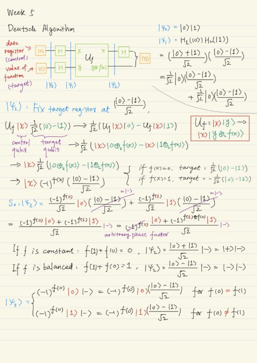
Deutsch Algorithm
Consider a boolean function f: {0,1}n → {0,1}. The domain of this function D(f) consists of 2n various n-bit sequences. The range of the function E(f) contains only two elements: 0 and 1.
| f is: | If: |
| constant | f(x) = 0 ∀x ∈ D(f); or f(x) = 1 ∀x ∈ D(f) |
| balanced | for 2n/2 values of x, f(x) =0; and for the other 2n/2 values of x, f(x) =1 |
Consider a special case when n = 1. The domain of f is 1 bit, and the range of f is also 1 bit. Then this problem can be reduced to calculating (f(0) + f(1)) MOD 2.
| f is: | because: |
| constant | (f(0) + f(1)) MOD 2 = 0 |
| balanced | (f(0) + f(1)) MOD 2 = 1 |
Let the function f(x) be either constant or balanced, we do not know in advance which of these two classes it belongs. Deutsch Problem is to determine which of these two classes the function f(x) belongs to.
| The classical approach | Solve the problem after calculating 2n/2 + 1 of its values. |
| The quantum Deutsch algorithm | Solve the problem after calculating only 1 value of f(x). |
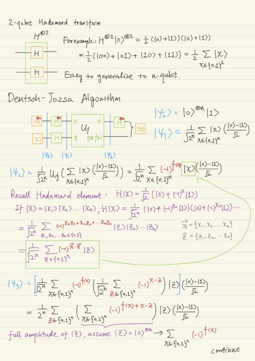
Deutsch-Jozsa Algorithm
Deutsch-Jozsa algorithm is the generalization of Deutsch algorithm, when n > 1. The first n-qubits in state |0⟩⨂n are used to prepare various argument values of the function f, with the help of the n-qubit Hadamard element H⨂n. The last qubit in the state |1⟩ is used to create the corresponding relative phase factor, to create the necessary quantum interference between the corresponding states after the transformation Uf.
If the function f(x) is constant, then after measuring the states of the data register, all its qubits will be in the state |0⟩. Otherwise, the function will be balanced.
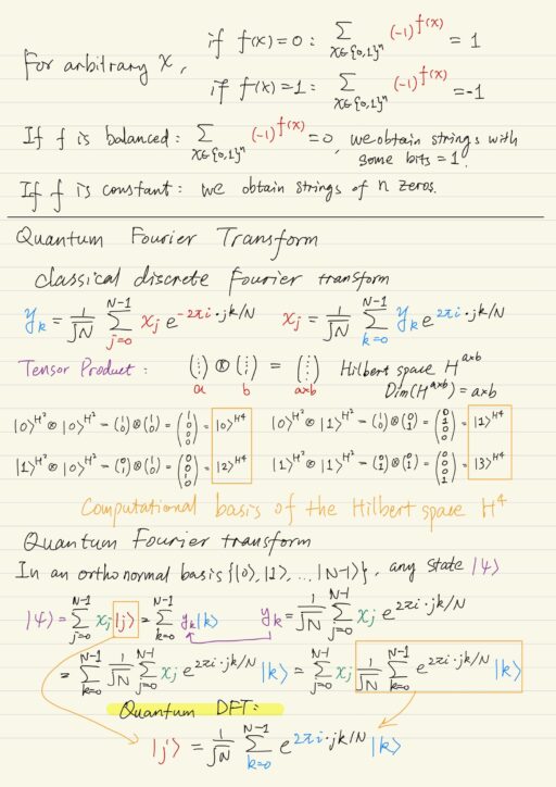
Quantum Fourier Transform
In mathematics, discrete Fourier transform (DFT) is widely used in digital signal processing algorithms. DFT requires a discrete function (as input) or a sample of values from a continuous function: {x0, x1, ..., xN-1}. As a result of the DFT, another discrete function is obtained {y0, y1, ..., yN-1}.
The direct discrete Fourier transform is defined as:
yk = 1/√N ∑N-1j=0 xj e-2πi*jk/NThe inverse discrete Fourier transform is defined as:
xj = 1/√N ∑N-1k=0 yk e2πi*jk/NThe quantum discrete Fourier transform is defined in the similar way, suppose in an orthonormal basis {|0⟩, |1⟩, ..., |N-1⟩}, the quantum direct Fourier transform is defined as:
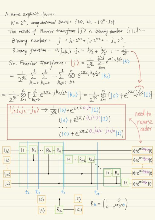
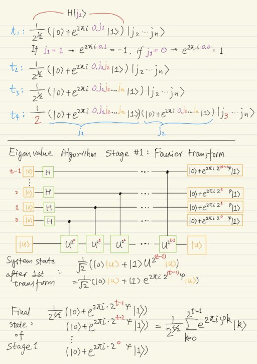
|j⟩ = 1/√N ∑N-1k=0 e2πi*jk/N |k⟩Suppose N = 2n, where n is a natural number. A more convenient form for implementation is:
|j⟩ = 1/2(n/2) ⨂nl=1 [|0⟩ + exp(2πi * j/2l) |1⟩]The quantum Fourier transform requires O(n2) operations, meanwhile the classical fast Fourier transform requires O(n 2n) operations. However this is not possible in practice due to the reduction postulate and measurement procedure.
Eigenvalue Algorithm
The quantum Fourier transform can be used to determine the eigenvalue of some unitary operator. Let a unitary operator U have an eigenvector |u⟩ and an eigenvalue e2iπφ, where φ is to be determined
To determine the eigenvalue, we will use controlled quantum logic gates capable of:
- preparing the state
|u⟩(the eigenstate of these quantum gates) and - performing the operation U^2j (U to the power 2 to the power j) for the non-negative j.
The procedure consists of 2 stages, each of which uses 2 registers:
- The first (data) register contains t qubits initially in the state |0⟩. The number of qubits t defines how accurately we want to determine the eigenvalue φ.
- The second (value) register contains as many qubits as needed for storing the state
|u⟩, and it is initial state is an eigenstate for the operator U. During the procedure, the state of the second register remains unchanged.
The first stage is nothing but the quantum Fourier transform of some initial state |ϕ⟩. Thus in order to calculate the phase ϕ, we need to perform the inverse quantum Fourier transform on the first register, as a result we obtain the state of |ϕ⟩ which will be given by a set of qubits in the state of |ϕ1⟩|ϕ2⟩...|ϕt⟩. This state will give a good estimation for ϕ, and therefore the eigenvalue of the unitary operator U, which correspond to its eigenstate |u⟩.
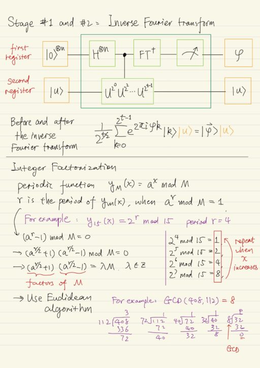
Integer Factorization
There are actual computational problems that can not be solved with the help of classical computers, such as the problem of factorizing large integers. The goal of the factorization algorithm is to determine primes factor p and q for a given integer M = p × q. Such a task is of great importance for modern classical cryptography or more precisely public key cryptographic systems, which generate and multiply two large primes to encode information. Since the primes are very large it is impossible to factor the result in number with ordinary computer in a reasonable time.
Factorization problem can be reduced to determining the order or the period r of a certain periodic function yM(x) = ax mod M, when ar mod M = 1, where:
x = 0, 1, ..., N-1;L = ⎡Log2N⎤is the number of bits needed for recording x;ais an arbitrary number that does not have common divisors with M, and 1 < a < M.
When the order r is known, the prime factors of a number M are determined using Euclidean algorithm as the greatest common divisor of numbers ar/2 ± 1 and M.
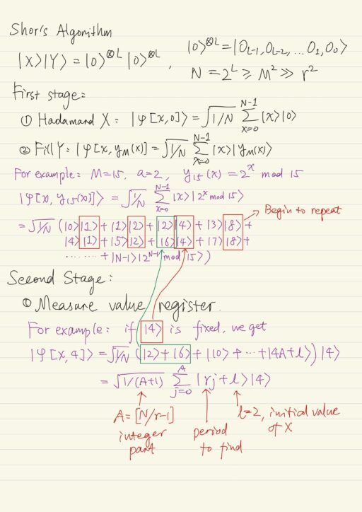
Shor’s Algorithm for Integer Factorization
To implement Shor’s algorithm, we use two quantum registers X (data) and Y (value), each of which consists of a set of L qubits in the |0⟩ state: |X⟩|Y⟩ = |0⟩⨂L|0⟩⨂L, here |0⟩⨂L = |0L-1, 0L-2, ..., 00⟩, and N = 2L ≥ M2 ≫ r2.
The register X contains the arguments (natural numbers) of the function yM(x), the register Y is used to keep the values of the function yM(x).
At the first stage:
- The state of the register X is transformed by Hadamard transforms into an equiprobable superposition of all Boolean states.
- Then the register Y is filled with values yM(x) = 2x mod M using a reversible logical operation, and a superposition is obtained.
At the second stage:
- Measure the value register in the measurement basis, and data register is still unmeasured. Thus the second register is used to prepare periodic superposition in the first register.
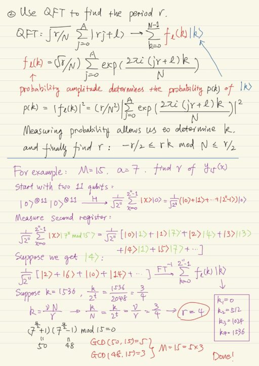
- Now we can find the period r using the Fourier transform which is performed on the state of the first (data) register.
- Then knowing the period r, we use the classical Euclidean algorithm.
Shor factorization algorithm gives an exponential gain in speed in comparison with the classical factorization algorithms.
My Certificate
For more on Quantum Algorithms, please refer to the wonderful course here https://www.coursera.org/learn/physical-basis-quantum-computing
Related Quick Recap
I am Kesler Zhu, thank you for visiting my website. Check out more course reviews at https://KZHU.ai