Quantum entanglement acts as a cornerstone for all quantum computations. If one physical system consists of two or more qubits and its state vector |ζ⟩ can be represented as tensor product |ζ⟩ = |ζ1⟩ ⨂ |ζ2⟩, where |ζ1⟩ and |ζ2⟩ describe states of each qubit. Then the state |ζ⟩ is called separable; otherwise it is called inseparable or entangled.
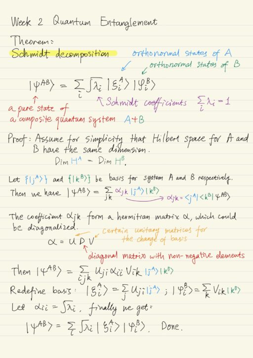
Theorem: Schmidt Decomposition
Let |ψAB⟩ be a pure state of a composite quantum system A + B, then there exists a set of orthonormal states {|ξiA⟩} of the system A and a set of orthonormal states {|φiB⟩} of the system B such that:
|ψAB⟩ = ∑i √λi |ξiA⟩ |φiB⟩where {√λi} are called the Schmidt coefficients and are non-negative real numbers, such that ∑i λi = 1. Using this theorem, we could find out whether a pure state is separable or entangled. The number of non-zero Schmidt coefficients {√λi} is called the Schmidt number. In other words, the Schmidt number is the number of terms in the Schmidt decomposition.
| If Schmidt number is | The pure quantum state of the composite system is |
| = 1 | Separable. The composite system state vector can be represented as a tensor product of state vectors corresponding to each part of the system.|ψAB⟩ = |ξA⟩ ⨂ |φB⟩ |
| > 1 | Entangled. |
Bell States (Einstein–Podolsky–Rosen Pairs)
Bell states act as a resource for superdense coding and quantum teleportation. The relative phase and parity define each of the Bell states. In order to define the four Bell states, one needs two classical bits. It also means one can transfer two bits information using the Bell states.
|β00⟩ = 1/√2 |00⟩ + 1/√2 |11⟩
|β01⟩ = 1/√2 |01⟩ + 1/√2 |10⟩
|β10⟩ = 1/√2 |00⟩ - 1/√2 |11⟩
|β11⟩ = 1/√2 |01⟩ - 1/√2 |10⟩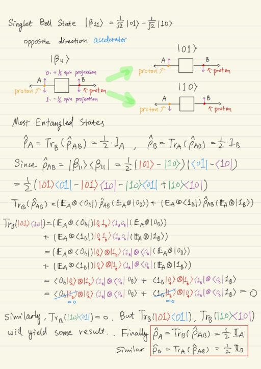
For example: we could prepare a system in the bell state |β11⟩, and have the spin projection of one particle A measured, then there is no need to measure the spin projection of anther particle B. The quantum states of these two particles appear to be differently interconnected. Here in the example of |β11⟩, the state of A and B particles are anti-correlated, since the spin projection values always appear to be opposite to each other: if one particle has a spin projection of +1/2, then the second one will have the spin projection value -1/2.
Similarly one could setup experiments for a system prepared in other Bell states. One will observe correlations between particle states.
Moreover, the Bell states are the most entangled states possible for a system of two qubits, which means if one takes a partial trace of the system density matrix over the states of the qubit B in order to obtain the density operator for the qubit A, we will get:
ρ^A = TrB(ρ^AB) = TrB(|βij⟩⟨βij|) = 1/2 IA
ρ^B = 1/2 IB
This means the result of our measurement is absolutely random: we will find the qubit A in a state |0⟩ with probability 1/2 or in a state |1⟩ with the same probability after the measurement. Thus we will not obtain any information about the prepared state after a local measurement of A or B qubit.
The four Bell states {|βij⟩} form an orthonormal basis for a two qubit Hilbert space. This means that any state vector of the two qubits quantum system can be represented in the form of Bell states superposition.
Entangled States
Entangled states manifest correlations which do not have any classical physics analogues. The intrinsic feature of these correlations is their non-locality. This means that the entangled particles can be distanced far away from each other, but the correlations will still exist and manifest themselves in physical experiments.
In order to entangle the pair of quantum systems, one should bring them into interaction with each other (done directly or using an auxiliary system). One should perform a certain collective unitary transform on the composed system.
EPR Paradox
The Bell states (EPR pairs) for a certain time have been serving as a basis for the critique of quantum mechanics ideas. Einstein, Podolsky and Rosen suggested the so-called EPR Paradox, which forced one to doubt all postulates of quantum theory. Nowadays quantum theory is generally accepted at least within it applicability limits. Quantum mechanics describes microword events perfectly.
Difficulties of quantum mechanics:
- The absence of determinism (jokingly being named as “the eviction of Laplace’s demon”). Quantum mechanics is built on probabilistic description of microscopic objects, so random processes are its intrinsic part.
- The observable object’s properties depend on the observation facilities. In quantum mechanics the observing instrument acts as a reference system; the micro object’s properties can not be described without any information on instruments with which they have been measured.
Simultaneous measurability
The values of the observables become determined directly after being measured with a physical instrument. The measuring instrument that measures an observable L, decomposes a state vector |ψ⟩ of any microsystem into a superposition of the measuring instrument’s eigenstates {|i⟩}. These eigenstates are macroscopically distinguishable: |ψ⟩ = ∑i ci|I⟩. The states |i⟩ and |i'⟩ are distinguishable if the condition ⟨i|i'⟩ = δii' holds.
Suppose two measuring instruments, corresponding to the observables L and M, have a common basis {|i⟩}, then [L^, M^] = 0 (commute). The observable L and M can be measured with the dispersion of zero, i.e. they are simultaneously measurable.
If two operators, corresponding to the observables L and M, do not commute, i.e. [L^, M^] ≠ 0, then these observables can NOT be measured simultaneously with the dispersion of zero. In other words: after every new measurement one will obtain a new random result.
Einstein, Podolsky and Rosen raised a concept called ‘hidden variable’ to questioned the quantum theory:
- Is it possible for non-commuting observables of a quantum system to exist simultaneously?
- Is it possible even if these observables can not be measured simultaneously with any existing measuring apparatus?
- In other words: do the “hidden variables” exist in a physical system?
In order to find out which one of these conceptions is objective (hidden variables or quantum theory), a special experiment was designed. The two conceptions shall make different predictions on the result of such an experiment.
This experiment can be realized by checking the so-called Bell inequalities. The Bell inequalities hold if the hidden variables conception is correct and they are violated if the quantum theory is right.
Bell Inequalities
John Bell suggested an idea of an experiment that allows one to check the correctness of both theories. Bell inequalities are understood as a set of experiments, which allow us to compare the predictions of hidden variables conception and quantum mechanics predictions.
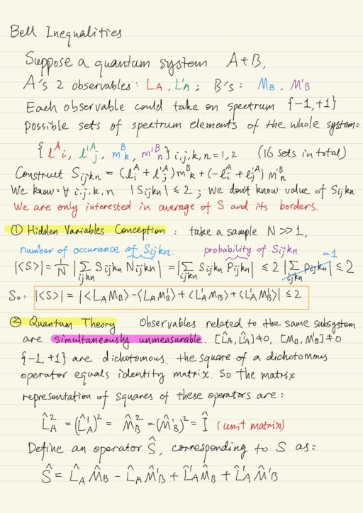
Suppose a compound quantum system A + B, that consists of A and B subsystems. Let LA and L'A be two observables of the subsystem A and MB, M'B be two observables of the subsystem B. Consider a simple spectrum {-1, +1} for each observable.
If all four observables occur to be the elements of physical reality (according to Einstein’s assumption), i.e. even if their values can not be measured due to an instrument’s imperfections, but these eigenvalues are fundamentally possible, then there exists (with non-negative probability) a set of their spectrum’s elements {lAi, l'Aj, mBk, m'Bn}, which could have been obtained after the measurement if possible.
Construct an observable S which depends on the observable LA, L'A, MB, M'B and define its corresponding operator S^. Hidden variables conceptions and Quantum theory give us different predictions:
| Hidden variables | CHSH inequality (the form of a Bell inequality)|⟨S⟩| ≤ 2 |
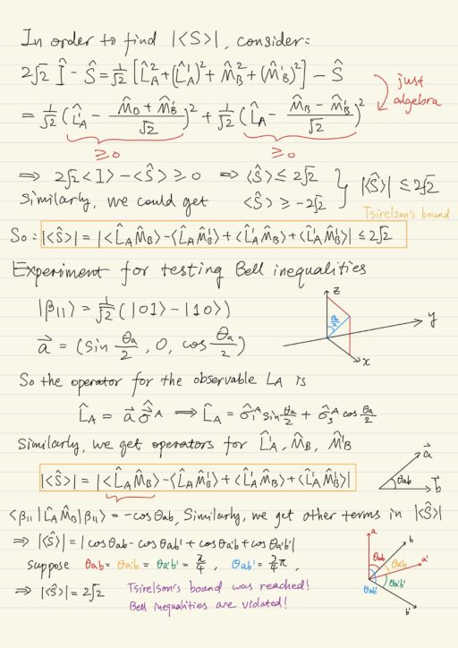
| Quantum theory | Tsirelson’s bound|⟨S^⟩| ≤ 2√2 |
If one obtained in experiment the value for 2 < |⟨S⟩| ≤ 2√2, then the Bell inequalities are violated and the Quantum Theory predictions occur to be correct. Otherwise, if |⟨S⟩| ≤ 2, then the Bell inequalities are obeyed and the hidden variables conception is true.
In the Bell test experiment, |⟨S^⟩| reaches the Tsirelson’s bound 2√2 at the parameters θab = θa’b = θa’b’ = π/4 and θab’ = 3π/4. Thus the Bell inequalities are violated. It means that the results predicted by the hidden variables conception occur to be wrong. On the contrary, results obtained in quantum mechanics approach are consistent with the experiment results. This demonstrates that non-local quantum correlation characteristics of the quantum entangled states contribute into the |⟨S^⟩|.
My Certificate
For more on Quantum Entanglement, please refer to the wonderful course here https://www.coursera.org/learn/physical-basis-quantum-computing
Related Quick Recap
I am Kesler Zhu, thank you for visiting my website. Check out more course reviews at https://KZHU.ai