Wave-particle Duality
The double-slit experiments show us:
| particle source | P1 : probability pattern when slit 1 is open P2 : probability pattern when slit 2 is open P12 = P1 + P2 : probability when both slits are open |
| wave source | (intensity of wave I is defined by its amplitude a) I1 = |a1|2 : when slit 1 is open I2 = |a2|2 : when slit 2 is open I12 ≠ I1 + I2 : when both slits are open, the two waves interfere with each other producing alternating maximum and minimum called “interference pattern” I12 = |a1 + a2|2 = I1 + I2 + 2√(I1I2)cosδ δ is the phase difference between a1 and a2 |
| electron source | 1. electron behaves like a particle when measured by a movable detector 2. electron behaves like a wave when both slits are open, even when electrons are shot one at a time P1 = |ψ1|2, P2 = |ψ2|2, P12 = |ψ1 + ψ2|2 |
The wave-particle duality is the peculiar property of a quantum mechanical particle that allows it to behave simultaneously like a particle and a wave.
Wave function and Born’s postulate
The quantum mechanical explanation for this phenomenon is to use a wave function ψ(r) to describe electron. The wave function represents the probability of finding an electron at a certain position. More specifically the absolute value square of the wave function |ψ|2 represents the probability.
P = |ψ|2 ensures the probability is positive number and it is also consistent with the electromagnetic theory, in which squared amplitude a of an electromagnetic wave is defined to be the intensity I of the electromagnetic wave.
| Electromagnetic theory | The complex amplitude of the electromagnetic wave indicates the magnitude and the phase of that particular field of the electric or magnetic. These complex notation in the electromagnetic theory is really a mathematical convenience. |
| Quantum mechanics | The wave function is fundamentally a complex quantity. The wave function itself has no analogue in the classical physics, this is a uniquely quantum mechanical quantity. |
P = |ψ|2 is also called the probability density, because it is actually probability per unit volume. For an infinitesimal volume dr around r, then the probability of finding an electron within that small volume dr located at r is proportional to the absolute value square of the wave function times the infinitesimal volume, i.e.: ∝ |ψ(r)|2 dr.
The sum of such probabilities should equal to unity, in other words, integrating the probability density |ψ(r)|2 across the entire space should be equal to 1.
∫ |ψ(r)|2 dr = 1 (normalized condition)The wave function, which satisfies the normalized condition, is called a normalized wave function. And the wave function can be normalized simply by multiplying a complex constant.
de Broglie’s matter wave
Wave length λ is related to momentum p of particles, where h = 6.626 × 10⁻³⁴ (Js) is Planck’s constant:
λ = h / pTime-Independent Schrödinger Equation
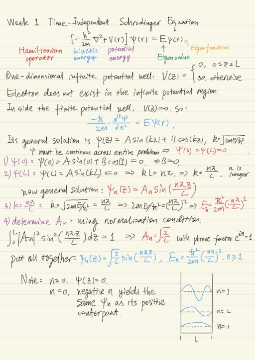
[-h2/2m ∇2 + V(r)] ψ(r) = E ψ(r)The equation is essentially defined by the Hamiltonian operator which represents energy inside the bracket. The first term -h2/2m ∇2 represents the kinetic energy, and the second term V represents potential energy. The goal is to solve this Eigenvalue equation to obtain the Eigenfunction ψ and the Eigenvalue E simultaneously.
The 1-dimensonal infinite potential well problem
One dimensional infinite potential well is defined by this potential profile:
V(z) = 0, 0 ≤ z ≤ L, L is the length of the well
V(z) = ∞, otherwise
An electron can not exist in the “infinite potential” region, also in this region the wave function ψ(r) = 0. In the “finite potential” region, since V(z) = 0, the time-independent Schrödinger equation is simplified:
-h2/2m ∂2ψ/∂z2 = E ψ(r)Its general solution is given as below, we need to use boundary condition to determine A, B and E.
ψ(z) = A sin(kz) + B cos(kz), k = √(2mE/h2)Wave function ψ has to been continuous across the entire problem, particularly at the well boundaries 0 and L, so ψ should be 0 at these boundaries:
ψ(0) = ψ(L) = 0The eigensolution of the problem is:
ψn(z) = √(2/L) sin(nπz/L)
En = h2/2m (nπ/L)2
n ≥ 1
There are a few non-classical behavior we can notice:
- Discrete set of allowed energies. Energies are quantized.
- The lowest possible (zero-point) energy E1 is not zero.
- Particles are not uniformly distributed throughout the well, and distribution is different for different energies. Because the ψ is describe by sin function, so |ψ|2 won’t be uniform.
Properties of Eigensolutions
Eigenvalues En and eigenfunctions ψn(z) combined are called eigensolutions. You may have more than one eigenfunctions associated with the same eigenvalue. For a given eigenvalue if you have multiple eigenfunctions, we call that degeneracy, or we say that the system has degeneracy. The number of eigenfunctions associated with the same eigenvalue is also referred to as the degeneracy.
One key property of eigenfunctions of the infinite potential well problem is parity. The parity is the symmetry about the center of the well. All of the eigenfunctions are either even or odd with respect to the center of the potential well. It is because the potential profile V(z) itself is symmetric about the center of the potential well. This parity is one of the most important characteristics in quantum mechanics that have impacts on a wide variety of physical phenomena.
The eigenfunctions En of the infinite potential well are really the basis set of a Fourier series. You can express an arbitrary function f as a linear combination of sine functions. The set of coefficient cn is called representation.
f(z) = Σ∞n=1 cn ψn(z) = Σ∞n=1 cn √(2/L) sin(nπz/L)The eigenfunctions are also orthogonal to one another. The orthogonality between functions (also the inner product of functions) is defined by this integral ∫∞-∞ g*(z)f(z) dz = 0, where * means taking complex conjugate. In the case of infinite potential well problem, you can easily demonstrate using the trigonometric function properties this:
∫L0 ψm*(z)ψn(z) dz = 0 for m ≠ n where ψn(z) = √(2/L) sin(nπz/L)The only case that this integral is not zero is when m and n are equal to each other: ∫L0 |ψn(z)|2 dz = 1. In general this could be compressedly expressed using Kronecker delta symbol:
∫L0 ψm*(z)ψn(z) dz = δmnIf a set of functions are orthogonal to one another and every single function is normalized, we call that an orthonormal basis set. Then it makes very easy to evaluate the expansion coefficients. All coefficients in the linear expansion can be used to construct a column vector. Here the eigenfunctions serve as the unit vectors and coefficients as the coordinates in geometric vector space.
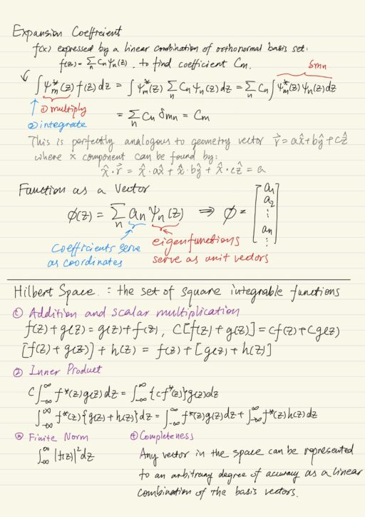
Hilbert Space
Square integrable functions meaning that if you take an absolute value of the function and square it, and if you integrate that absolute value squared over the entire space, it gives you a finite number, it doesn’t diverge. The set of square integrable functions form a vector space called Hilbert space. Each of these square integrable function is actually a vector in this vector space.
Any vector function in the space can be represented to an arbitrary degree of accuracy, meaning that there is no approximation, this is precisely equal. You can take any function in the space, and then you can express it as a linear combination of basis vectors.
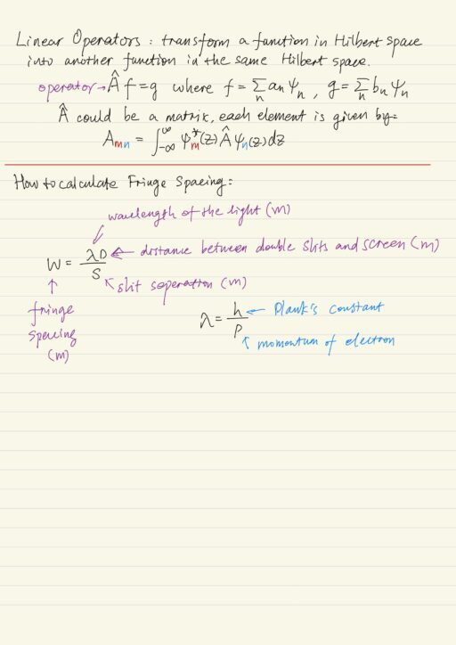
Linear operators transform a function (a vector) in Hilbert space into another function (vector) in the same Hilbert space. A linear operator can be represented by a matrix.
My Certificate
For more on Time-Independent Schrödinger Equation, please refer to the wonderful course here https://www.coursera.org/learn/foundations-quantum-mechanics
Related Quick Recap
I am Kesler Zhu, thank you for visiting my website. Check out more course reviews at https://KZHU.ai