The mathematical model of quantum computing allows us to understand and design quantum algorithms without any background in quantum mechanics or physical implementation of quantum hardware. The most significant part of the whole theory of quantum computing is qubit, i.e. quantum bit, which is the minimum unit of quantum information. One qubit information can be encoded by polarization of a photon or the orbital of electron in the hydrogen atom.
Qubit
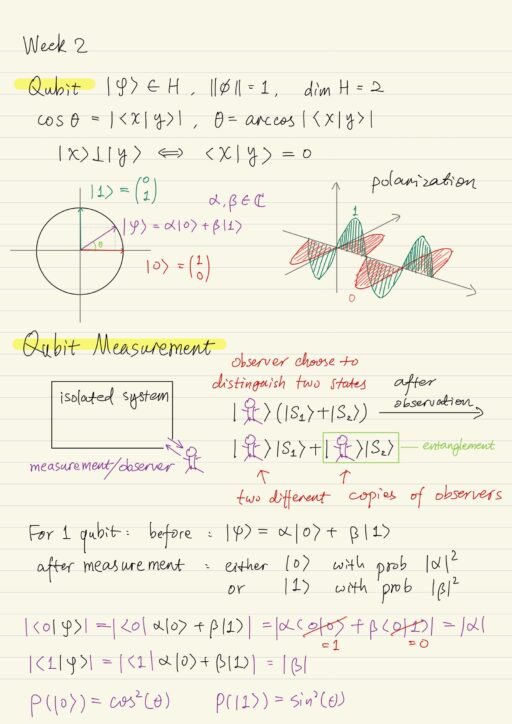
The strict mathematical definition of a qubit is “a unitary vector in a two-dimensional Hilbert space”.
|φ⟩ ∈ H, ||φ|| = 1, dim H = 2Hilbert space is a linear space over some field with a dot (or inner) product. We usually only focus on the finite dimensional spaces over the field of complex numbers C. if you have two vectors: XT= [x1, ..., xn] ∀xi ∈ C, and yT = [y1, ..., yn] ∀yi ∈ C, then their dot (inner) product will be:
⟨x|y⟩ = ∑nj=1 x*j∙yjwhere |y⟩ (called ket) is a column vector, and ⟨x| (called bra) is a transposed vector (row vector) of conjugated coordinators x*i. This definition of inner product satisfies:
⟨x|y⟩ = ⟨y|x⟩*
⟨x|x⟩ ≥ 0
⟨x|αy + βz⟩ = α⟨x|y⟩ + β⟨x|z⟩
The cosine of the angles between two qubits cos(θ) = |⟨x|y⟩|, two qubits are orthogonal to each other |x⟩⊥|y⟩ if and only if ⟨x|y⟩ = 0. In a unitary circle, the vertical unitary vector (from center to the upper) |1⟩ and the horizontal unitary vector (from center to the right) |0⟩, form the orthonormal basis in the space. This unitary circle is the all possible values of one qubit. So one qubit can not be only |0⟩ or |1⟩, but it can be any vector on this unitary circle |φ⟩ = α|0⟩ + β|1⟩ α,β ∈ C.
Two Qubits
In the overwhelming majority of case, we need more than 1 qubit to perform computation. Imaging we have two particles each carrying one qubit |0⟩ or |1⟩, it is convenient for us to describe the system in Hilbert space over complex numbers. But this space has to be four dimensional. Each measurement outcome will be again one of the basis vectors (|00⟩, |01⟩, |10⟩, |11⟩) of this space.
Before measurement, if a qubit is in superposition, we can still describe the system using the basis we just constructed.
| qubit 1 | qubit 2 | system |
| |0⟩ | α |0⟩ + β |1⟩ | α |00⟩ + β |01⟩ P(|00⟩) = |α|2, P(|01⟩) = |β|2 |
| α |0⟩ + β |1⟩ | γ |0⟩ + δ |1⟩ | αγ |00⟩ + αδ |01⟩ + βγ |10⟩ + βδ |11⟩ P(|01⟩) = |αδ|2 = |α|2|δ|2 Sum of all of the square of coefficients equals 1. |
There are states like 1/√2 (|00⟩ + |11⟩) that are physically exist but can not be constructed through the process above. Note the real quantum systems, the qubits, they don’t situate in some Hilbert spaces. It is just our way of describing them.
We usually use tensor product to derive the column representation for basis vectors.
|00⟩ = |0⟩ ⨂ |0⟩ = [1 0]T ⨂ [1 0]T = [1 0 0 0]T
|01⟩ = [0 1 0 0]T
|10⟩ = [0 0 1 0]T
|11⟩ = [0 0 0 1]T
This rule is very convenient because the ket uses binary notation, say 10 is the binary notation of 2, to indicate the position of the single ‘1’ in the column vector is 2 (the third place), all other positions are zeros.
More Qubits
In a system with n qubits, we will have a Hilbert space with 2n dimensions. A system with 1000 particles is described by about 10300 complex numbers.
Qubit Measurement
The choice of this orthonormal basis seems arbitrary, but is needed for the measurement of the qubit. Quantum systems are isolated systems, the measurement / observation does not alter the state of the system, instead it records the information about the system into the observer and alters the wave function of the observer.
Before observation, the observer can choose the states he is going to distinguish, by the choice of the basis or the choice of observable operator.
After observation, we have two different copies of observers, each of them entangles with one of these states, observing different state of the system. Observer subjectively obtains one of the basis vectors as the measurement outcome. This is how measurement happens from the multiverse’ point of view.
From the interpretation of multiverse point of view, when we say a system is in state |φ⟩ = α|0⟩+ β|1⟩, we mean among all the snapshots / copies of the universe which contains this state, the mean value of this state is |φ⟩. It does not mean that in every universe, this state is exactly vector |φ⟩, it is a mean value over all the copies of the universe. The shares of each copy in the whole multiverse are defined by coefficients α and β.
Measurement is destructive, after the very first measurement, the system jumps to the basis vector that we obtained as a measurement of outcome. If we perform measurements for multiple times, we obtain always the same result. Also no-cloning theorem tells us that copying of unknown quantum state is impossible.
Hadamard Basis
If you don’t know anything about the quantum state, then the measurement will give us very little information about it. But if we do know something, we can attune the measurement process to obtain more information.
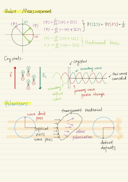
For example, assume we know our quantum state is either |φ⟩ = 1/√2 (|0⟩ + |1⟩) or |ψ⟩ = 1/√2 (- |0⟩ + |1⟩), if we still use |0⟩ and |1⟩, then the measurement of this qubit will give us zero additional information, because for both of the state, the probability of outcome |0⟩ or |1⟩ are the same 1/2.
Hadamard basis is defined as:
|+⟩ = 1/√2 (|0⟩ + |1⟩)
|-⟩ = 1/√2 (|0⟩ - |1⟩)
these 2 vectors are orthogonal and unitary, so they form orthonormal basis. If we measure the quantum system in this basis. Then the result |+⟩ will tell us the system was in and is still in state |φ⟩, and |-⟩ outcome tells us the system was in |ψ⟩ before the measurement. So choosing the correct basis is crucially important for obtaining information from quantum system.
Polarizers
Polarization is the direction of the wave oscillation, which is orthogonal to the direction of wave propagation. Crystals can be used to detect and alter the polarization. Crystals contain dipoles which are all oriented along one axis.
If we apply alternating electromagnetic field E→ with the vector of oscillation parallel to this axis. Then the charged particles ⊕ ⊖ began to oscillate around the position of the minimum of potential energy. And those oscillating charged particles produce waves. This secondary wave will be shifted half of the period to the primary wave (if the primary wave is sinusoidal). The primary and secondary waves cancel each other, so actually there is no wave passed the crystal.
On the contrary, if we have the primary wave polarized along the prorogation direction, then it does not cause oscillations of the charged particles, so it does not produce the secondary wave, and the primary wave easily passes the crystal. The axis which shows the waves to pass is called the optical axis of the crystal. The light that pass through the polarizer is polarized along its optical axis.
So this is why some materials are not transparent for some wavelength. If inside the material there is some charged particles which can oscillate with a frequency of the primary wave (falling into the material), then this charged particles produces secondary waves which then destroys the primary wave. So the primary wave does not pass through this material and thus fully reflected. For example all metals are not transparent for all most all frequency of the electromagnetic waves because of free electrons. And they are also shiny because of the reflected waves.
Almost all transparent materials alter the light polarization, so if you put something transparent between two crossed polarizers. then the light, which came through the transparent material can NOW pass the second restriction polarizer, because the polarization was slightly changed. If there is any area with higher density in the transparent material, we will have more light which was not restricted by the second polarizer. Thus we can analyze the defect in the transparent material, which we don’t see in normal light.
The polarizer can perform the measurement process for us for the light polarization, and the choice of the basis is performed by rotation of the polarizer.
Entanglement in Multiple Qubit Systems
There are famous representatives of a set of states which are called the Bell states. They exist or can be implemented, but can not be constructed using the tensor product as described in previous sector.
1/√2 (|00⟩ + |11⟩)
1/√2 (|01⟩ + |10⟩)
These Bell states describe some state of a system on 2 particles, however the state of each individual particle can not be described – these particles don’t have separate states. They are in some sense entangled. Suppose a system was in state 1/√2 (|00⟩ + |11⟩), if the measurement of the first qubit gives the result |1⟩, then |00⟩ is removed, we immediately know the second qubit will have state |1⟩. The second qubit’s state is entangled with the first qubit, it is impossible for it to have other states.
This can be explained using the multiverse interpretation of quantum mechanics.
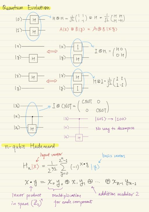
More than storing qubits, we need to modify qubits to do computation. Any modification (represented by a operator) must be unitary. The unitary operator is a linear operator for which its adjoint is also its inverse. The matrix of an adjoint is the conjugate transpose of the matrix of the original operator.
U U* = U* U = I
U* = U-1
Unitary operators preserve the length of the vectors, also preserve the angles, thus the inner product.
|| U |x⟩ || = || x ||
| ⟨ U |x⟩ | U |y⟩ ⟩ | = | ⟨x|y⟩ |
Some examples include Hadamard operator, X (NOT) operator, CNOT (conditional NOT) operator.
My Certificate
For more on Mathematical Model of Quantum Computing, please refer to the wonderful course here https://www.coursera.org/learn/quantum-computing-algorithms
Related Quick Recap
I am Kesler Zhu, thank you for visiting my website. Check out more course reviews at https://KZHU.ai