Role of Statistics
Statistics is the study of systems that exhibit variability. Because macroscopic systems are composed of atoms and molecules that are in constant motion, what we see at the macroscopic level are averages of that variability.
Suppose we knew the kinetic energy of every molecule in a volume, then the average kinetic energy per molecule would be E = 1/N ∑Ni=1 ϵi. However there are just too many particles, we can not know all the energies, instead what we are able to determine are probability distributions of energies.
Probability distributions are functions that describe the likelihood or probability of finding a particle in a given state. Distributions can be discrete or continuous. x is the variable of interest, the probability of finding a value of x between limits a and b are given by summing or integrating over the probability distribution function from a to b.
| Discrete | Rotation, vibration, electronicP(a < x < b) = ∑ba f(x) dx |
| Continuous | Velocity or speedP(a < x < b) = ∫ba f(x) dx |
Distributions have some important integral properties, if a distribution function (pdf) is normalized, then its integral is unity ∫+∞-∞ f(x) dx = 1. Then we have moments of the distribution function: mean and variance. In principle, there are infinite number of moments, and if all the moments were known, the distribution function could be recovered.
| Mean | x- = ∫+∞-∞ f(x) dx |
| Variance | V = ∫+∞-∞ (x - x-)2 f(x) dx |
Josiah Willard Gibbs made the following observations:
- Matter is made up of large number of particles.
- There is a difference between the time average behavior of a single system and the average behavior of a large number of systems at an instant in time.
The physics of the situation are:
- There are large number of particles (atoms and molecules) in practical systems.
- The particles have kinetic and potential energy and are constantly in motion (center of mass translation, vibration, rotation, electronic motion).
- Particles and systems are constantly changing quantum state. Atoms and molecules will exist in discrete dynamic states called quantum states. Particle quantum states and system quantum states are distinct. The system quantum state is the state for which all the particle quantum states are specified.
- Either particle or system quantum states are those allowed by the macroscopic constraints (conservation of energy).
- Dynamics preclude most allowed states from appearing within reasonable observation times. It takes time for quantum states to change.
- Since equilibrium is observed, most observed states must look familiar. Thus equilibrium system quantum states must be more likely to occur than non-equilibrium ones.
One way to find the equilibrium quantum state is to look at the relative probability of each allowed state, and characterize equilibrium with the most probable allowed quantum state. Thus we must find the distribution of quantum states that is most probable.
Traditionally, there are two methods to find the most probable allowed quantum states:
- Watch a single system and look at all the allowed state. This requires that we assume that all allowed states are equally likely to appear (which is not the case).
- Watch a large number of systems each subject to the same conditions. If the number of systems is large enough, all allowed quantum states can appear (but which is physically unrealistic).
Gibbs chose the second method. An ensemble (a closed overall system) is a collection of identical systems (called members). The reservoirs (which contain the members) are so large that the associated intensive properties (T, p, μ) are held constant in all members. All members are subject to the same conditions, constraints, and allowed interactions.
Once we know the quantum state distribution function, we can calculate the average (expectation value, denoted using symbol ⟨ and ⟩ in statistics) of mechanical properties internal energy U, volume V and moles Ni:
⟨A⟩ = 1/n ∑j nj Aj
n - total number of ensemble members
j - ensemble member quantum state index
nj - number of ensemble members in quantum state j
Aj - U, V or Ni
Postulates of Microscopic Thermodynamics
Postulate 1
The macroscopic value of a mechanical-thermodynamic property of a system in equilibrium is characterized by the expected value computed from the most probable distribution of ensemble members among the allowed ensemble member quantum states.
This postulate merely state one can calculate ⟨A⟩ using the most probable distribution, i.e. 1/n n*j = p*j, which is the most probable probability distribution and * means the most probable.
⟨A⟩ = 1/n ∑j n*j Aj = ∑j p*j AjPostulate 2
The most probable distribution of ensemble members among ensemble member quantum states is that distribution for which the number of possible quantum states of the ensemble and reservoir is a maximum.
Postulate 2 describes how to determine the most probable distribution. To apply the postulate, we must obtain an express for the number of allowed quantum states as a function of the nj. Then find the nj that maximized the function.
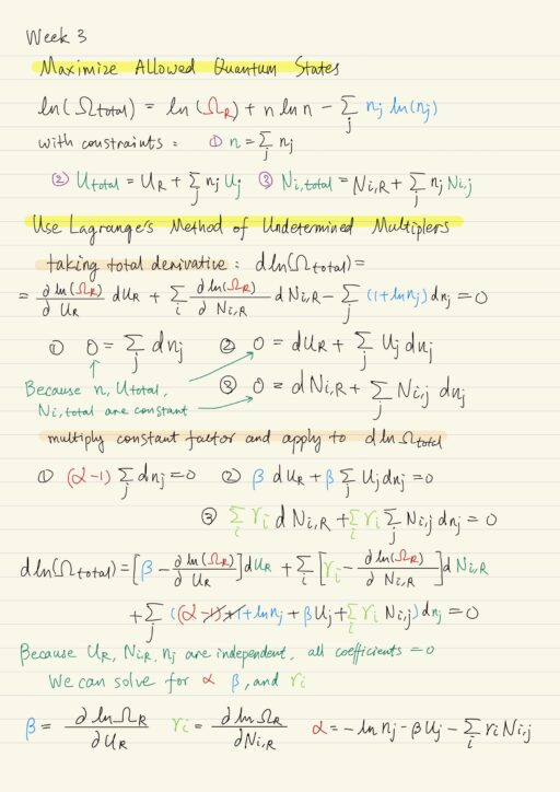
Allowed Quantum States
For an ensemble involving a reservoir, the members are in some quantum state, the reservoir are in another state. The total number available to the entire ensemble including the reservoir is:
ΩTotal = Ω ∙ ΩR
Ω - number of states available to the members
ΩR - number of states available to the reservoir
It turns out that we don’t need ΩR, but we will need an expression for Ω in terms of nj. But how many ways (permutations) can n members in a given distribution of quantum states be arranged? It is Ω = n! / ∏j nj!. Such total number of states is:
ΩTotal = ΩR ∙ n! / ∏j nj!
Due to Stirling’s approximation, ln(x!) = x ln(x) - x, if x >> 1, it turns out that it will be easier if we work with the log of Ω:
ln(ΩTotal) = ln(ΩR) + n ln(n) - n - (∑j nj ln(nj) - nj)
= ln(ΩR) + n ln(n) - (∑j nj ln(nj))
Out task now is to find the set of nj that maximizes this function. To begin, we need to select a type of ensemble, Microcanonical, Canonical, Grand Canonical, any will work well.
| Gibb’s Name | Independent Parameters | Fundamental Relation |
| Microcanonical | U, V, Ni | S(U, V, Ni) |
| Canonical | 1/T, V, Ni | S[1/T] |
| Grand Canonical | 1/T, V, -μi/T | S[1/T, V, -μi/T] |
For the Grand Canonical representation, we fix 1/T and -μi/T using reservoirs of energy and mass. Also fixing the total number of ensemble members we get a constraint: n = ∑j nj.
Recall that the allowed quantum states are those that satisfy conservation of energy, etc. So we have these 2 more constraints below, where Uj is the energy associated with state j; and Ni,j is the number of type i particle associated with state j. These will be finally determined eventually using quantum mechanics.
UTotal = UR + ∑j nj Uj
Ni,Total = Ni,R + ∑j nj Ni,j
The math problem that we have is to maximize a function subject to constraints. This turns out to be pretty simple using Lagrange’s Method of Undetermined Multipliers. At last we get the expression as the most probable distribution:
pj = 1/n n*j = exp(- βUj - ∑i γiNi,j) / ∑j exp(- βUj -∑i γiNi,j)Partition Functions
The denominator QG(β,γi) ≡ ∑j exp(- βUj -∑i γiNi,j) plays a very important role in thermodynamics. It is called the Partition Function. It allows us to determine, for an equilibrium state, how the quantum state of a system are partitioned or distributed.
The Lagrange multiplier β and γi are associated with Uj and Ni,j respectively. It turn out to be this, where k is Boltzmann’s constant.
β = ∂lnΩR/∂UR = 1/kT
γi = ∂lnΩR/∂Ni,R = -μi/kT
Partition Functions can be represented in alternative forms. Above, we derived Grand Canonical form, but it could have done the same for other representations.
| Gibb’s Name | Independent Parameters | Partition Function | Fundamental Relation |
| Microcanonical | U, V, Ni | Q = Ω | S(U, V, Ni) |
| Canonical | 1/T, V, Ni | Q = ∑j exp(-Uj/kT) | S[1/T] |
| Grand Canonical | 1/T, V, -μi/T | Q = ∑j exp(-Uj/kT + ∑i μi/kT Ni,j) | S[1/T, V, -μi/T] |
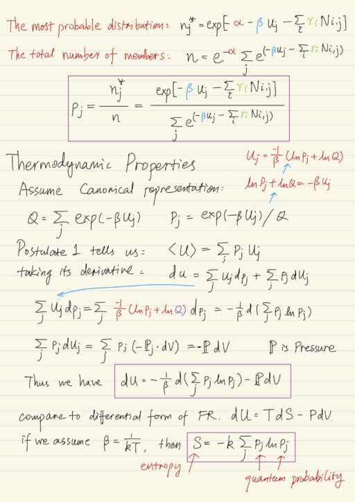
Thermodynamic Properties
A very important finding that relates entropy and quantum probability:
S = -k ∑j pj ln(pj)If we substitute the expression for pj into it, when S = 1/T U + k ln(Q). Compare this with the definition of S[1/T] = S - 1/T U, thus we have S[1/T] = k ln(Q), now we have directly related the Fundamental Relation to the partition function Q. This expression turns out to be valid in any representation, so in general:
S[...] = k ln(Q)Fluctuations
Fluctuations are consequences of the statistical behavior at the microscopic level. We have taken a statistical approach, the physics allow variability in state between ensemble numbers, or equivalently in time for a single system. Variability is small however it exists.
Consider the variance of an extensive property A, and symble ⟨ and ⟩ mean expectation value. The variance can be written in terms of the probability distribution pj.
σ2(A) ≡ ⟨ (A - ⟨A⟩)2 ⟩ = ∑j pj(Aj)2 - ⟨A⟩2For example, the variance of energy in the Canonical representation:
σ2(U) = ∑j pj(Uj)2 - ⟨U⟩2Quantum Statistics
Partition Function
We now make the connection between quantum mechanics and the macroscopic properties through the partition function. Two limiting cases are considered: electrostatic interactions between particles are neglected or allowed.
| Neglected | For most of the time, particles are unaffected by the presence of other particles. Collisions or other interactions that change the quantum state of a given particle DO occur, but rapidly, so that at any given time we can assume that all the particles are in stationary quantum states. (Ideal gases) |
| Allowed | (Liquids, solids, and dense gases) |
We need to make important distinction between ensemble member quantum state and particle quantum state. The former is the state specified by the latter.
| Uj | Energy of ensemble member in quantum state j. |
| Nj | Number of particles in ensemble member in quantum state j. |
| Ui,j | Energy associated with type i particle of member in quantum state j. |
| Ni,j | Number of i type particle in member in quantum state j. |
| Ni,k | Number of i type particle in particle quantum state k. |
| εi,k | Energy of i type particle in particle quantum state k. |
| Ni,k,j | Number of i type particle in particle quantum state k in member in quantum state j. |
| i | Particle type index |
| j | Member quantum state number |
| k | Particle quantum state number |
In the Grand Canonical representation, we are concerned with the ensemble number energy Uj and particle numbers Nj:
Uj = ∑i Ui,j = ∑i ∑k εi,k Ni,k,j
Nj = ∑i Ni,j = ∑i ∑k Ni,k,j
The partition function thus becomes below. The summation over j is over all possible ensemble member quantum states. A possible member quantum state is specified completely by specifying a value for each of the Ni,k,j.
Q = ∑j exp(-β Uj - ∑i γi Ni,j)
= ∑j exp(- ∑i ∑k (β εi,k + γi) Ni,k,j)
= ∑j ∏i ∏k exp[-(β εi,k + γi) Ni,k,j]
Quantum mechanics will give us Ni,k and εi,k. Since the Grand Canonical system is open, there are no constraints placed, by the surfaces surrounding the ensemble members, on the possible values of the Ni,k,j‘s. Thus one can remove ∑j, and replace specification of all possible values and combinations of the Ni,k,j‘s and write:
Q = ∏i ∏k ∑MaxNi,kη=0 exp[-(β εi,k + γi)η]where MaxNi,k is the maximum number of i type particle which may simultaneously occupy the k-th particle quantum state. The advantage of this form for the partition function is that the sum is for a single quantum state of a single type particle.
Pauli Exclusion Principle
The behavior of particles is described by a wave function. The symmetry properties of the wave function play a role in the behavior of systems of particles. Suppose the coordinates of two indistinguishable particles are reversed. The sign of the wave function may or may not change depending on the type of particle:
| Sign | Change | Not change |
| Wave function | Anti-symmetric | Symmetric |
| MaxNi,k | 1 | Infinity |
| Particle name | Fermion | Boson |
| System name | Fermi-Dirac | Bose-Einstein |
| Examples | Deuterium, Helium3, Electrons | Hydrogen, Helium4, Photons |
The partition functions for fermions and bosons become:
QFD,BE = ∏i ∏k (1 ± exp[-β εi,k - γi])±1
ln QFD,BE = ∑i ∑k ln(1 ± exp[-β εi,k - γi])±1
Maxwell-Boltzmann Limit arises when the density is so low that the issue of symmetry is no longer important, i.e. exp[β εi,k + γi] >> 1. The number of molecules in the Maxwell-Boltzmann Limit is given by the relatively simple expression:
⟨N⟩MB = ∑i ⟨Ni⟩ = ln(QMB) = ∑i ∑k exp[-β εi,k - γi]This limit is important because it leads to the ideal gas law. So:
S[...] = k ln(Q) = PV/T
⟹ PV = NkT
For those instances where the Maxwell-Boltzmann Limit does not apply, the thermodynamic behavior is strongly influenced by whether the particles are bosons or fermions.
My Certificate
For more on Statistical Thermodynamics, please refer to the wonderful course here https://www.coursera.org/learn/macroscopic-microscopic-thermodynamics
Related Quick Recap
I am Kesler Zhu, thank you for visiting my website. Check out more course reviews at https://KZHU.ai