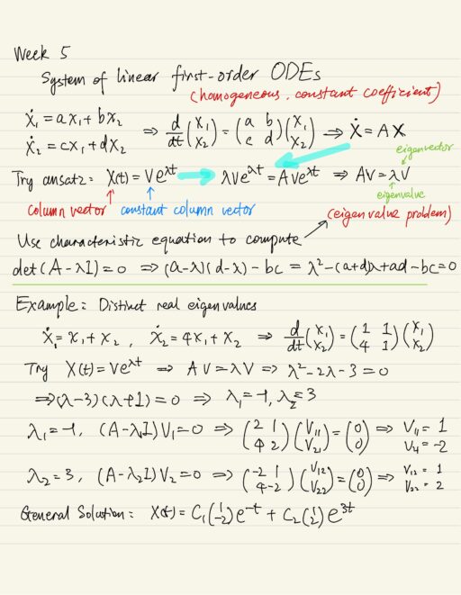
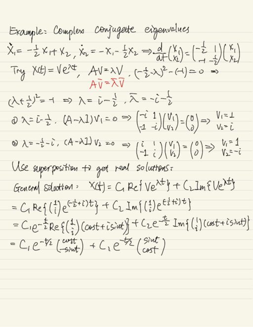
Systems of Homogeneous Linear First-order ODEs
The system of linear first order homogeneous equations can be written in matrix form. To solve it we’re going to use
- An ansatz
X(t) = V eλt. We’re going to look for solutions of the ansatz. - The principle of superposition. When we find solutions of the ansatz, we’ll multiply them by constants and add them together to get the general solution.
Substituting the ansatz into the differential equations, we get an eigenvalue problem A V = λ V . We could use the characteristic equation det( A - λ I ) = 0 to calculate eigenvalue λ . There are 3 probable things happen:
- two distinct real values
- complex conjugate roots
- repeated degenerated roots
When you have a complex eigenvalue and a complex eigenvector, you have a complex solution of the differential equation, we would like to have two real solutions, so we can use the usual principle of superposition.
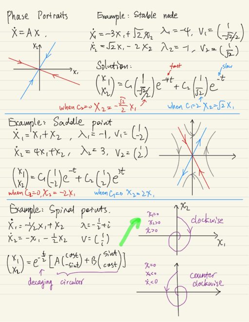
Phase Portraits
The diagrams called phase portraits are used to visualize the solution of the equation X' = A X, and the visualization is done in what’s called the phase space of the solution. The origin of the graph (0, 0) value is called a fixed point or equilibrium point, which means that if the solution starts at (0, 0), i.e. if the initial condition for X was (0, 0) then it stays at (0, 0) for all time, because the derivative X’ is 0.
| Stable | all nearby solutions will be attracted to the equilibrium. |
| Unstable | all solutions will run away from the equilibrium. |
We solve the differential equation by putting some initial condition (a point on the diagram) and we follow where this point moves in the phase space. We will then draw diagrams for several initial conditions surrounding the origin ( fixed point) and see what the diagram looks like.
The qualitative nature of the solutions will depend on the eigenvalues and the eigenvectors of the matrix A.
| Eigenvalues | Solutions | Fixed point |
| 2 distinct real, both negative | Decaying exponential behaviors Trajectories converge onto the origin | Stable node |
| 2 distinct real, both positive | Growing exponential behaviors Trajectories running away from the origin | Unstable node |
| 2 distinct real, one negative, one positive | Along one of the eigenvectors, the solution is going into the origin Along another eigenvector the solution is running away from the origin | Saddle point |
| Complex, negative real part | Stable spiral | |
| Complex, positive real part | Unstable spiral |
A saddle point is unstable because as long as you have a non-zero value of constant coefficient C2, the initial condition is not exactly on the line when C2 = 0, then eventually the solution will go to infinity.
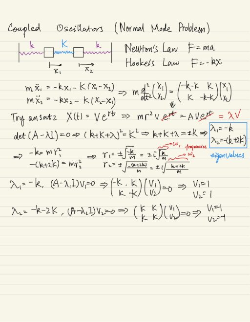
Normal Mode Problem
Normal mode problem is a model example which will show the power of analyzing a system of equations using eigenvalues and eigenvectors. In the example of couple of oscillator, the motion doesn’t look simple but in fact it is simple, the random motion of 2 masses is simply a superposition of these two simple motions:
- The first normal mode has a frequency of the
√(k/m), is when the masses are both moving together to the right and to the left. - The second normal mode has a frequency of
√((k + 2K)/m), and it’s when the two masses are moving opposite each other.
My Certificate
For more on Systems of Differential Equations, please refer to the wonderful course here https://www.coursera.org/learn/differential-equations-engineers
Related Quick Recap
I am Kesler Zhu, thank you for visiting my website. Check out more course reviews at https://KZHU.ai